2025-06-02
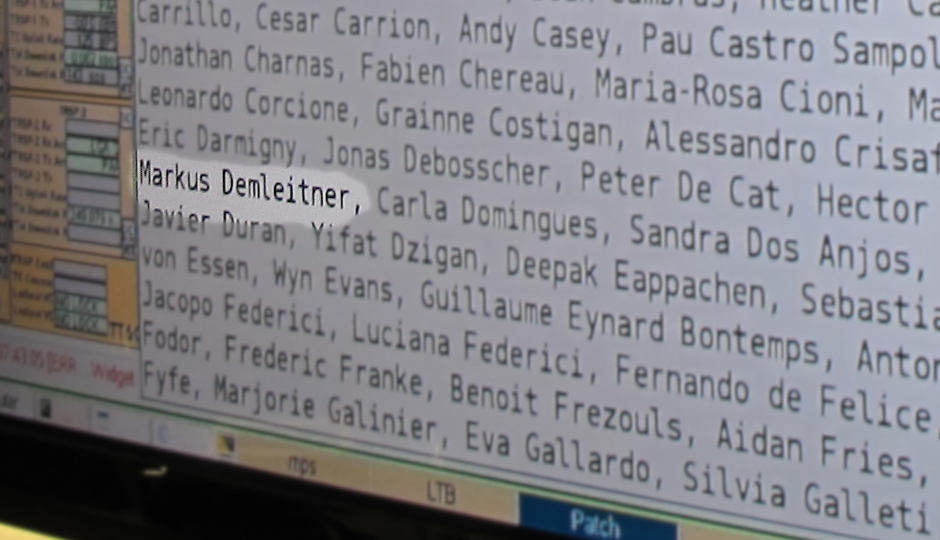
Markus Demleitner
A bit more than six months after the Malta Interop, the people
working on the Virtual Observatory are congregating again to discuss
what everyone has done about VO matters and what they are planning to
do in the next few months.
Uneasy Logistics
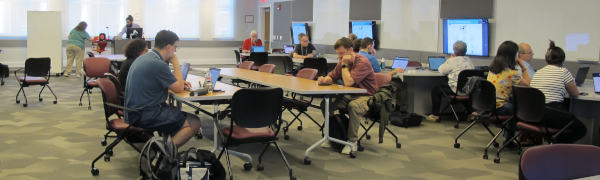
This time, the event takes place in College Park, Maryland, in the metro
area of Washington, DC. And that has been a bit of an issue with
respect to “congregating”, because many of the regular Interop attendees
were worried by news about extra troubles with US border checks. In
consequence, we will only have about 40 on-site participants (rather
than about 100, as is more usual for Interops); the missing people have
promised to come in via some proprietary video conferencing system
<cough>, though.
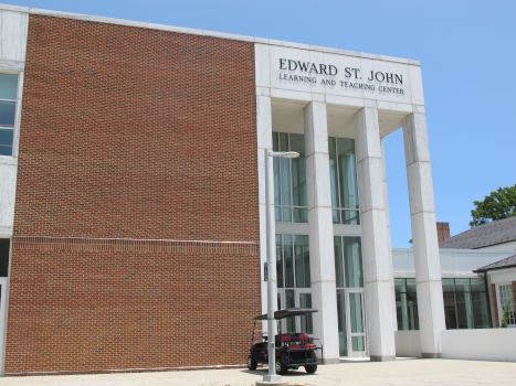
Right now, in the closed session of the Technical Coordination Group,
(TCG) where the chairs of the various Working and Interest Groups of
the IVOA meet, this feels fairly ok. But then more than half of the
participants are on-site here. Also, the room we are in (within the
Edward St. John Learning and Teaching Center pictured above) is
perfectly equipped for this kind of thing, what with microphones in each
desk, and screens everywhere.
I am sure the majority-virtual situation will not work at all for what
makes conferences great: the chats between the sessions. Let's see how
the usual sessions – that mix talks and discussion in various
proportions – will work in deeply hybrid.
TCG: Come again?
The TCG, among other things, has to worry about rather high-level,
cross-working-group, and hence often boring topics. For instance, we
were just talking about how to improve the RFC process, the way we
discuss whether and how a draft standard (“Proposed Recommendation”)
should become a standard (“Recommendation”). This, so far, happens on
the Twiki, which is nice because it's stable over long times (20 years
and counting). But it also sucks because the discussions are hard to
follow and the link between comments and resulting changes is loose at
best. For an example that should illustrate the problem, see the last
RFC I ran.
Since we're sold to github/Microsoft for our current document
management
anyway, I think I would rather have the RFC discussions on github,
too, and in some
way we will probably say as much in the next version of the Document
Standards. But of course there are many free parameters in the
details, which led to quite a bit more discussion than I had expected.
I am not entirely sure whether we sometimes crossed the border to bikeshedding;
my hope is we did not.
Here's another example of the sort of infrastruture talk we were having:
There is now a strong move to express parts of our standards' content
machine-readably in OpenAPI (example for TAP). Again, there are
interesting details: If you read a standard, how will you find the
associated OpenAPI files? Since these specs will rather certainly
include parts of other standards: how will that work technically (by
network requests or in a single repository in which all IVOA OpenAPI
specs reside)? And more importantly, can a spec say “I want to include
a specific minor version of another standard's artefacts“?
Must it be minor version-sharp, and how
would that fit with semantic versioning? Can it say “latest”?
This may appear very far removed from astronomy. But without having
good answers as early as possible, we will quite likely repeat the mess
we have had with our XML schemas (you would not believe how much
curation went into this) and in particular their versioning. So,
good thing there are the TCG sessions even if they sometimes are a bit
boring.
Now that I think of it: In our XML schema, we now implicitly always say
“latest for the major version”, and I think that has served us well. I
should have mentioned that a prior art for this question.
Opening session (2025-06-02, 14:30)
The public part of the conference has started with Simon O'Toole's
overview over what was going on in the VO in the past semester.
Around page 36 of his slide set, updates from the Rubin Observatory
say what I have been saying for a long time:
If you don't understand what they are talking about, don't worry too
much: It's a fairly technical detail of writing VOTables, where we did a
fix of something rather severly broken in 2012.
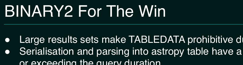
The entertaining part about it, though, is that later in the conference,
when I will talk about the challenges of transitioning between
incompatible versions of protocols, BINARY2 will be one of my examples
for how such transitions tend to be a lot less successful than they
should be. Seeing takeup by players of the size of Rubin almost proves
me wrong, I think.
Charge to the Working Groups (2025-06-02, 15:30)
This is the session in which the chairs of the Working and Interest
Groups discuss what they expect to happen in the next few days. Here is
the first oddity of what I've just called deeply hybrid: The room we
are in has lots of screens along the wall that show the slides; but
there is no slide display behind the local speaker:
If you design lecture halls: Don't do that. It really feels weird when
you stand in front of a crowd and everyone is looking somewhere else.
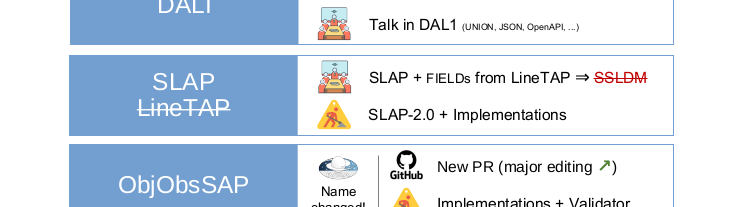
Content-wise, let me stress that this detail from Grégory's DAL talk
was good news to me:
This means that the scheme for distributing spectral line data that
Margarida and I have been working on for quite a while now, LineTAP
(last mentioned in the Malta post), is
probably dead; the people who would mostly have to take it up, VAMDC,
are (somewhat rightly) scared of having to do a server-side TAP
implementation. Instead, they will now design a parameter-based
interface.
Even though I have been promoting and implementing LineTAP for quite a
while, that outcome is fine with me, because it seems that my central
concern – don't have another data model for spectral lines – is
satisfied in that that parameter-based interface (“SLAP2”) will build
directly upon VAMDC's XSAMS model, actually adopting LineTAP's proposed
table schema (or something very close) as the response table. So,
SLAP2, evolved in this way, seems like an eminently sensible compromise
to me.
Tess gave the Registry intro, and it promises a “Spring Cleaning
Hackathon” for the VO registry. That'll be a first for Interop, but one
that I have wished for quite a while, as evinced by my (somewhat
notorious) Janitor post from 2023. I am fairly sure it will be fun.
Data Management Challenges (2025-06-03, 10:30)
Interops typically have plenary sessions with science topics, something
like “the VO and radio astronomy”. This time, it's less sciency, it's
about “Data Management” (where I refuse to define that term). If you
look at the session programme, in it
some major science projects will be telling you about
their plans for how to deal with (mostly large) new data collections.
For instance Euclid, has to deal with several dozen petabytes, and they
report 2.5 million async TAP queries in the three months from March,
which seems incredibly much. I'd be really curious what people
actually did. As usual: if you report metrics, make sure you give the
information necessary to understand them (of course, that will usually
mean that you don't need the metrics any more; but that's a feature, not
a bug). In this case, it seems most of these queries are the result of
web pages firing off such queries when they are loaded into
Javascript-enabled web browsers (or crawlers).
More relevant to our standards landscape, however, is that ESA wants to
make the data available within their, cough, Science Data Platform,
i.e., computers they control and that are close to the data. To exploit
that property, in data discovery you need to somehow make it such that
code running on the platform can find out file system paths rather than
HTTP URIs – or in addition to them? We have already discussed possible
ways to address such requirements in Malta, without a clear path forward
yet that I remember. Pierre, the ESA speaker, did not detail their
plan.
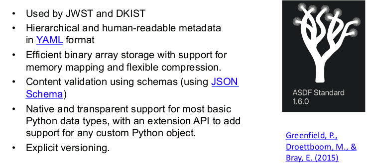
In the talk from the Roman people, I liked the specification of their
data reduction pipeline (p. 8 ff); I think I will use this as a
reference for what sort of thing you would need to describe in a full
provenance model for the output of a modern space telescope. On the
other hand, this slide made me unhappy:
Admittedly, I don't really know what use case the pre-baked table files
that they want to serve in this ADSF format are supposed to
cover, but I am rather sure that efficiency-wise having Parquet files
(which they intend to use elsewhere anyway) with VOTable metadata as per Parquet
in the VO would not make much of a difference.
But it would bring them much closer
to proper VO metadata, which to me sounds like a big win.
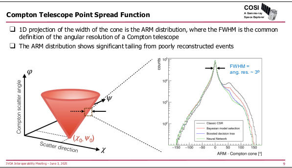
The remaining two talks in the session covered fairly exotic
instruments: SphereX, which scans the sky into a giant spectral cube, and
COSI, a survey instrument for MeV gamma rays (like, for instance:
60Fe, which is a strong signal in Supernovae)
with the usual challenges for making something like an
image out of what falls out of your detector, including the fact that
the machines' point spread function is a cone:
How exciting.
Registry (2025-06-03, 12:30)
I'm on my home turf: The Registry Session, in which I will talk about
how to deal with continuously updated resources. But before that,
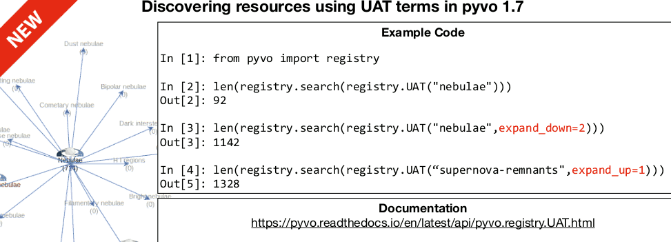
Renaud, the current chair of the Registry WG, pointed out something I
did (and reported on here): Since yesterday, pyVO 1.7 is out and
hence you can use the UAT constraint with semantics built-in:
Ha! The experience of agency! And I'm only dropping half a smiley here.
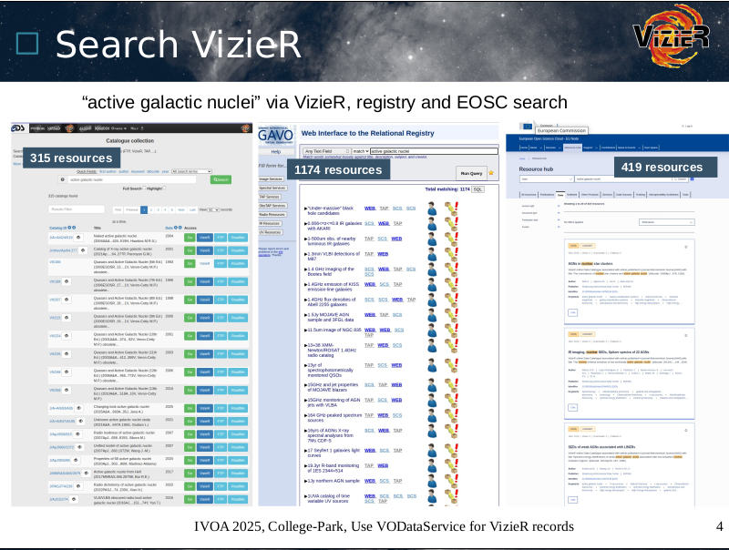
Later in the session, Gilles reported on the troubles that VizieR still
has with the VOResource data model since many of their resources contain
multiple tables with coordinates and hence multiple cone search
services, and it is impossible in VODataService to say which service is
related to which table. This is, indeed, a problem that will need
some sort of solution. I, for one, still believe that the right solution
would be to fix cone search rather than try and fiddle together some
sort of kludge (and I don't see anything but kludges on that side) in the
Registry.
He also submitted something that could be considered
a bug report. Here are match counts for three different
interfaces on top of (hopefully) roughly equivalent metadata
collections:
I think we'll have to have second and third looks at this.
Tuesday (2025-06-03) Afternoon
I was too busy to blog during yesterday's afternoon sessions, Semantics
(which I chaired in my function as WG chair emeritus because the current
chair and vice chair were only present remotely) and then, gasp, the
session on major version transitions. The latter event was mainly a
discussion session – that worked rather well in its deeply hybrid form,
I am happy to report –, where everyone agreed that (a) as a community, we
should be able to change our standards in ways that break existing
practices lest we become sclerotic and that (b) it's a difficult thing
and needs careful and intensive management.
In my opening pitch, I mentioned a few cases where we didn't get the
breaking changes right. Let's try to be better next time. At
the session, some people signalled they would be in on updating Simple Cone
Search from the heap of outdated legacy that it now is into an elegant
protocol nicely in line with modern VO standards (which certainly would
be a breaking change). Now, if only I could bring myself to imagine the
whole SCS2 business as something I would actually want to do.
If you are reading this and feel you would like to pull SCS2 along with
me: Do write in.
Let me remark that I found it a stellar moment of this session when a
former Google employee mentioned that at Google they did think long
and hard about whether to kill Reader (which was supporting
the open RSS standard, and thus was a positive thing at least by Google
standards) and then decided they would not
keep running it for three people in a cave.
Ummm, now that I think
about it, I don't remember whether the ”three people in a cave” quip
came from her, but somehow the phrase was in the room, and one
participant actually got fairly cross because they are missing Google
Reader to this day and they resented being considered one of
three people in a cave.
Similarly for the “breaking change“ of switching mobile phone standards
(GSM to UMTS to LTE), there were immediately people in the room who are
still unhappy because they had to discard perfectly good phones when the
networks their modems knew were shut down. So, in a way my message of
“if you can help it, don't do breaking changes, because someone will
get pissed with you” was brought home very impressively. This one time,
however, I'd much rather be wrong. Perhaps there are ways to have
relatively painless major version migrations of more or less mature
federated systems.
Raising some hopes in that direction,
the migration from Plastic to SAMP in the early days of the VO was mentioned as
something that has worked rather nicely. Ok: That was not exactly a
federated client-server system, but it was not too far from that either.
Perhaps one should have a closer look at that story.
DCP (2025-06-04, 10:00)
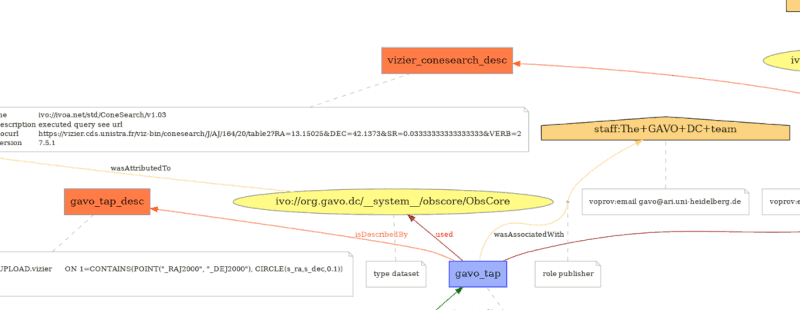
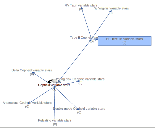
I'm now sitting the the session of the Data Curation and Preservation
WG, and I am delighted that in Gilles' talk, something that was, in
the end, rather simple in implemenation yields something as complex as
provenance graphs such as this:
which occurs towards the end of Gilles' slideset. The full graph
integrates our part of a not entirely trivial table's provenance with
some metadata coming from CDS. That I found remarkable in itself.
The delightful detail about it, however, is that I had never planned for the
data origin implementation to enable anything like this. That on the
client side you can do things the publishers have never meant you to do
(and mind you, I personally am not convinced scientists would like to
contemplate such graphs), that is why I think interoperable standards
letting users do whatever they like on their end of the protocol is such
a great thing.
Yes, that was a stinger against “platforms”, as much they have been all
the craze a few years ago. On them, the publisher controls the client,
too, and the more platformy something is, the more users will be limited
by the ideas of the publishers.
Obscore and Extensions (2025-06-04, 15:00)
I was worried for a moment that this would be an Interop day without a
talk by me. Fortunately, Renaud asked me to give his talk on the
Registry aspects of Obscore extensions (which, to be fair, already had
me on its author list before). This is in the context of something I am
fairly happy about: extra tables next to instances of ivoa.obscore
(where we can store all kinds of results of astronomical observations)
that cover metadata that is peculiar to certain fields: messenger types
like radio or high energy for instance. If you are running DaCHS, you
can already have a draft of one of these (Radio) since DaCHS 2.10.
So, this time, there is a session on the extensions for high energy,
radio, and possibly time, with a view of how to
use and find them in practice. Given that the
unfortunate (“my biggest mistake”) dataModel element for discovery
of Obscore tables came up again in Grégory's talk, I am happy I had a
chance to make my point again on why we need to discover these kinds of
things differently than what I had envisioned in 2012. If you
weren't there: It's basically what I said last year in TableReg (the
April 2025 date on this reflects a very minor fix).
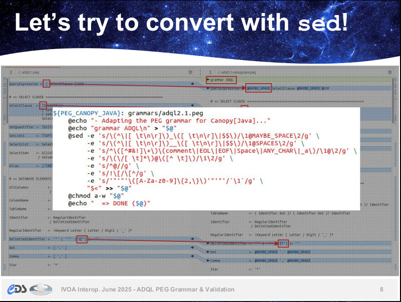
Apps II (2025-06-05, 12:00)
When I sat in the Apps 2 session I was still shaking my head about
Grégory's slide from his talk on rewriting the grammar for our ADQL
query language in a formalism called PEG. In itself, PEG and the
grammar are great (I have contributed to it quite a bit myself). They
give
absolutely no reason for head-shaking. But then there are various
libraries that read PEG grammars and build parsers from them. It
turns out that each library has tiny little, largely inexplicable quirks
in the way they expect the PEG to be written.
This made Grégory squeeze something like a source grammar through
several
pieces of sed horror to fit it to the various concrete PEG machineries.
Here's how this looks like for the Canopy PEG library:
Call me overly sensitive, but it's things like these that sometimes makes
me seriously consider becoming a vegetable gardener and don't ever touch
computers again.
But then I'm too much of a language lawyer to not enjoy the sort
nitpicking I just did in the Apps 2 session, and none of that would exist
without computers. Basically, it was about this VOTable being broken:
<VOTABLE><RESOURCE><TABLE>
<FIELD name="objname" datatype="char" arraysize="*"/>
<DATA><TABLEDATA><TR>
<TD>Joachim Wambsganß</TD>
</TR></TABLEDATA></DATA></TABLE></RESOURCE></VOTABLE>
Looks fine to you? Well, have a look at my lecture notes to see
what's wrong and what ways to improve the situation I see. Still, I
feel an urge to
confess I had quite a bit of rather twisted fun when I gave that talk.
It must be that kind of sentiment that leads to the Babylonoid confusion
that Grégory has regretted in his PEG talk.
DM 3 (2025-06-05, 17:00)
Another plenary discussion session: Data Models: modularity, levels,
endorsement. I have to really try hard not to blurt out “told you so,
told you so” every few minutes.
But I could not resist sneaking in a link to a PR against astropy that
still illustrates what I think we should to DMs like (even if it's now
many years old):
https://github.com/msdemlei/astropy. I think I'll leave this repo at
commit dcc88dc forever. And that's about all I can say about
that topic without losing my equanimity. Aw, I even had code showing
how to deal with breaking changes in that astropy fork:
pos_ann = None
for desired_type in ["stc3:Coords", "stc2:Coords"]:
  for ann in ann.get_annotations(desired_type):
    pos_ann = ann

    if pos_ann is not None:
      break

if pos_ann is None:
  raise Exception("Don't understand any target annotation")
Meanwhile, the Spring Cleaning Hackaton of the Registry WG that I had
looked forward to above happened two hours ago. It was very interesting
to debug the workflow for assigning subject keywords for resources (the
thing I was taking about in my lofty semantics post) for a certain
data centre that shall remain unnamed here. We eventually found out the
reason their subjects were substandard was that the person responsible
for picking them was not aware of that responsibility.
If you ask me, this hackathon showed again that getting people together
in a room is the preferred way to work out what these days you might
call hybrid problems: Not entirely social and organisational, but not
entirely technical either. What we did in that hour would have taken
many mails and a lot more time to solve if we had even started doing
it rather than just resigning to the (in this case) substandard
keywords.
Wrapping Up (2025-06-06)
I am sitting in the traditional last session of the Interop, where the
chairs of the various Working and Interest Groups look back on their
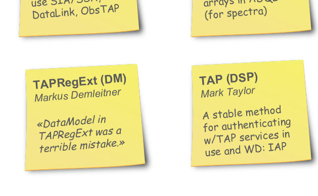
sessions. I just have to comment one thing from Grégory and Joshua's
summary for DAL, where they quote me as:
Let me stress that the reason I was so blunt here is that it was I who
put the dataModel element into TAPRegExt. It seemed a good idea at the
time. For the story of how that later turned out to be an mistake, I
would again like to draw your attention to TableReg.
Before this closing session, I had my last talk at this Interop. That
happened in the
DAL 2 session in the form of a report on my addition to the persistent
uploads that I have recently discussed here. The following talk by
Pat from CADC mentioned that they did the indexing part somewhat
differently; let's see how we reach consensus here.
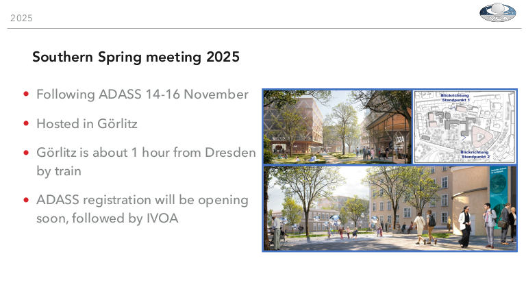
So, that's it for this Interop. The parting exec chair, Simon, had the
last word, rightfully thanking the local organisers who really had a hard
time given the political chaos around them, and also reminded people
that we will next meet in Görlitz – which means that I will be the local
organiser. I'm nervous already:

![[RSS]](./theme/image/rss.png)