![[RSS]](../theme/image/rss.png)
Limits, Materialisation, and Anchor Texts: DaCHS 2.13 is out

With all the crazy Star Trek-sounding talk of “materialising obscore” below I could not resist and asked stabledifffusion.com for „Thirteen badgers materialising obscore“. Well, counting badgers is hard, and I wouldn't have been sure how to visualise obscore, either. Rest assured, though, that the remainder of this post is not AI slop and at least factually correct.
It's been almost a year since the last release of our publication package, DaCHS, and so it's high time for DaCHS 2.13. I have put it into our repository last Friday, and here is the obligatory post on the major news coming with it.
Perhaps the biggest headline (and one that I'd ask you to act upon if you run a DaCHS system) is support for the new features in the brand-new VODataService 1.3 Working Draft. That is:
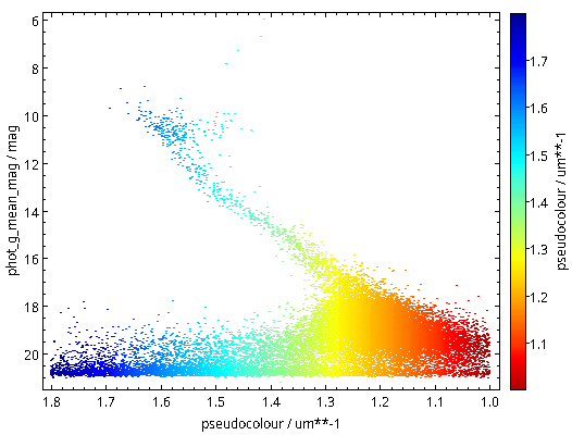
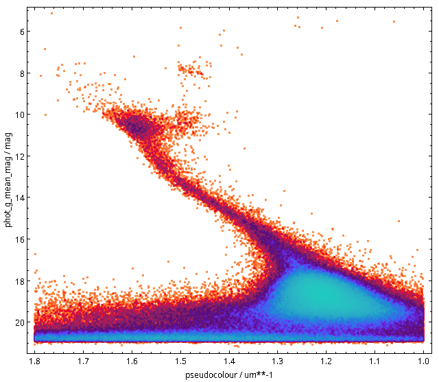
Column statistics. This is following my Note on Advanced Column Statistics on the way to improved blind discovery in the VO. To have them in your DaCHS, all you have to do is upgrade and run dachs limits ALL – and then make sure you run dachs limits after a dachs imp you are satisfied with (or use the new -l flag discussed below). Please do it – one can do a lot of interesting discovery in the Registry (and perhaps quite a bit more) if this is taken up broadly.
Product type declaration. So far, when you wanted to discover, say, spectra, you would enumerate the SSAP services in the Registry, perhaps with some additional constraints (e.g., on coverage), and then query each of those.
Linking data types and protocols was a reasonable shortcut in the early VO. It no longer is, for a whole host of reasons, among which Obscore (which can publish any sort of observational data) ranks pretty high up. So, in the future, we need to be explicit on what among the terms from http://www.ivoa.net/rdf/product-type will come out of a service.
Where this is immediately useful is when you publish time series through SSAP (which is not uncommon). Then, just put:
<meta name="productType">timeseries</meta>
into the root of your RD (the time series template in 2.13 already does this). If you publish cubes through SIAP, you should similarly say:
<meta name="productType">cube</meta>
For other SSAP and SIAP services, you probably don't need to bother at this point.
For obscore, DaCHS will do the declarations for you if you have run:
dachs limits //obscore
– which is a good thing to do anyway (see above).
Data source declaration. For most purposes, it is really important to know whether some piece of data you found is based on actual observations or whether it's data coming out of some sort of simulation.
So far, the only protocol that let you say something like that was SSAP. But there's now all kinds of other non-observational data in the VO, and so VODataService 1.3 introduces the vocabulary http://www.ivoa.net/rdf/data-source to let you say where the data you publish comes from.
The default is going to be observational for a long while. If that's what you have, don't bother. But if you publish results from simulations (more or less: starting from random numbers), put:
<metaName="dataSource">theory</metaName>
into your RD's root, and if it's data based on actual objects (simulated observations for a new instrument, say, or model spectra for concrete stars), make it:
<metaName="dataSource">artificial</metaName>
To make filling in the VODataService column statistics somewhat less of a hassle, I have added an -l flag to dachs imp. This makes it run (in effect) a dachs limits after the import. I'm not doing this on every import because that would slow down the development of an RD; obtaining the statistics may take quite some time, and for certain sorts of tables you may prefer to run dachs limits with your own options.
You could argue I should have inverted the logic, where you'd rather pass a flag saying “don't do limits” during development. You could probably convince me. But until someone protests, just remember to add an -l flag to your last import command.
There are a few more prototypes for (possibly) upcoming standards in DaCHS 2.13. For one, you can now write units in ADQL queries as per my proposal at the Görlitz ADASS. That is, you can annotate literals with units in curly braces (as in 10{pc}), and you can convert values with known units into other units using a new operator @. For instance, if you were fed up with the stupid angle unit we've been forced to accept since… well, about 2000 BC, you could put the interface to saner units into your queries like this:
SELECT TOP 20
  ra@{rad}, dec@{rad}, pmra@{rad/hyr}, pmdec@{rad/hyr}
FROM gaia.dr3lite
This is not a big advantage if you write queries just for a single catalogue. It does make a difference when you write queries that ought to work across multiple tables and services.
While you should not notice the per-mode limit declarations coming from an unpublished draft of TAPRegExt 1.1 (except that the async limits TOPCAT shows will now better match what DaCHS actually enforces), you could appreciate the support for StaticFile that comes out of DocRegExt 1.0. There, it is used to register single PDF files or perhaps ipython notebooks. When you register such things[1], you can now say something like:
<publish render="edition" sets="ivo_managed">
  <meta>
    accessURL: \internallink{\rdId/static/myfile.txt}
    accessURL.resultType: text/plain
  </meta>
</publish>
The result of this will be that DaCHS produces a doc:StaticFile interface rather than vs:WebBrowser, and it will produce a resultType element saying that what you get back is plain text (in this case). If you have other applications for having static files like that in registry records, do let me know.
My investigation into slow obscore queries I already reported on here led to two changes: For one, some types in the obscore table changed, and in consequence dachs val -vc ALL will complain when you pulled in the obscore columns into your own tables. Just try the val -vc and either re-import the affected resources at your leisure (it's only an aesthetic defect, things will continue to work) or change the column types as described in the blog post linked above.
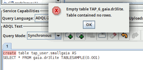
Probably more importantly, you can now materialise the obscore view (actually, in order to let you drop the contributing tables at will, it's not a materialised view but a table, but that's… immaterial here). You want to do that if you have many contributions to your obscore table, at least some queries against it become slow and you can't seem to figure out why. See Materialised Obscore in the tutorial to see what to do if you want to materialise your obscore table, too.
Something perhaps worth exploring for you is that you can now publish entire RDs. I implemented this for a resource with lots of little “services” (actually, HiPSes) that share so many pieces of metadata that it just seemed wrong to have them all separate resource records (though I am in discussion with the HiPS people who are not particularly fond of having multiple HiPSes in one resource record), nsns. Beyond that, you could have, say, a cone search for extracted sources, an image service and a browser service for both in one RD and then say, in the RD section with top-level metadata:
<publish sets="ivo_managed"/>
– everything should then live nicely as separate capabilities within one resource record and that without any of the publish/@service tomfoolery you had to use so far to glue together VO and browser services.
For local publications (i.e., browser services appearing on your front page), this will result in a link to the RD info (minor DaCHS secret: <your server URL>/browse/<rd-id> gives an overview over the tables and services defined in an RD). Whether that's useful enough for you in such a case I cannot predict. But you can mix all-RD publications in ivo_managed with conventional <publish sets="local"/> elements for browser services.
Among the more minor changes, the default web form template now employs a WebSAMP connector, which means that the SAMP button on results of the form renderer is now greyed out until a SAMP hub becomes visible on your machine.
If you use a display hint type=url, you can now control the anchor text on the a element in HTML output by setting a property anchorText on the corresponding column. Yes, that will then be constant for all the products. If you really need more control than that, you will have to define a formatter for a custom outputField.
So far, the fullDLURL macro could only be used when you actually had a normal, filename-based DaCHS access reference. This was unfortunate because this kind of thing is particularly convenient for “virtual” data generated on the fly. Hence, you can now pass some python code in a second fullDLURL argument that must return the accref to use. Read a bit more on the context in Datalinks as Product URLs.
There are many other minor changes and fixes that you hopefully will only notice because some annoying behaviour of DaCHS is now a little less annoying.
If you spot problems or miss something, feel free to report that at our new repository at Codeberg. The main VCS for DaCHS still is https://gitlab-p4n.aip.de/gavo/dachs. But we will probably migrate to Codeberg by the 2.14 release to make reporting bugs and writing pull requests simpler.
Perhaps we will receive some from you?
| [1] | Using resType: document; I notice I should really add some material on registering educational material with DaCHS to the tutorial. |