• Automating TAP queries

    TOPCAT is a great tool – in particular, for prototyping and ad-hoc analyses, it's hard to beat. But say you've come up with this great TAP query, and you want to preserve it, perhaps generate plots, then maybe fix them when you (or referees) have spotted problems.

    Then it's time to get acquainted with TOPCAT's command line sister STILTS. This tool lets you do most of what TOPCAT can, but without user intervention. Since the command lines usually take a bit of twiddling I usually wrap stilts calls with GNU make, so I just need to run something like make fig3.pdf or make fig3.png and make figures out what to do, potentially starting with a query. Call it workflow preservation if you want.

    How does it work? Well, of course with a makefile. In that, you'll first want to define some variables that allow more concise rules later. Here's how I usually start one:

    STILTS?=stilts
    
    # VOTables are the results of remote queries, so don't wantonly throw
    # them away
    .PRECIOUS: %.vot
    
    # in this particular application, it helps to have this global
    HEALPIX_ORDER=6
    
    # A macro that contains common stuff for stilts TAP query -- essentially,
    # just add adql=
    TAPQUERY=$(STILTS) tapquery \
      tapurl='http://dc.g-vo.org/tap' \
      maxrec=200000000 \
      omode=out \
      out=$@ \
      ofmt=vot \
      executionduration=14400
    
    # A sample plot macro.  Here, we do a healpix plot of some order. Also
    # add value_1=<column to plot>
    HEALPIXPLOT=$(STILTS) plot2sky \
      auxmap=inferno \
      auxlabel='$*'\
      auxvisible=true \
      legend=false \
      omode=out \
      out=$@ \
      projection=aitoff \
      sex=false \
      layer_1=healpix \
        datalevel_1=$(HEALPIX_ORDER) \
        datasys_1=equatorial \
        viewsys_1=equatorial \
        degrade_1=0 \
        transparency_1=0 \
        healpix_1=hpx \
        in_1=$< \
        ifmt_1=votable \
        istream_1=true \
    

    For the somewhat scary STILS command lines, see the STILTS documentation or just use your intution (which mostly should give you the right idea what something is for).

    The next step is to define some pattern rules; these are a (in the syntax here, GNU) make feature that let you say „to make a file matching the destination pattern when you have one with the source pattern, use the following commands”. You can use a number of variables in the rules, in particular $@ (the current target) and $< (the first prerequisite). These are already used in the definitions of TAPQUERY and HEALPIXPLOT above, so they don't necessarily turn up here:

    # healpix plots from VOTables; these will plot obs
    %.png: %.vot
          $(HEALPIXPLOT) \
                  value_1=obs \
                  ofmt=png \
                  xpix=600 ypix=380
    
     %.pdf: %.vot
           $(HEALPIXPLOT) \
                   value_1=obs \
                   ofmt=pdf
    
     # turn SQL statements into VOTables using TAP
     %.vot: %.sql
           $(TAPQUERY) \
                  adql="`cat $<`"
    

    Careful with cut and paste: The leading whitespace here must be a Tab in rules, not just some blanks (this is probably the single most annoying feature of make. You'll get used to it.)

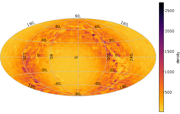
    What can you do with it? Well, for instance you can write an ADQL query into a file density.sql; say:

    SELECT
      count(*) as obs,
      -- "6" in the next line must match HEALPIX_ORDER in the Makefile
      ivo_healpix_index (6, alphaFloat, deltaFloat) AS hpx
    FROM ppmx.data
    GROUP BY hpx
    

    And with this, you can say:

    make density.pdf
    

    and get a nice PDF with the plot resulting from that query. Had you just said make density.vot, make would just have executed the query and left the VOTable, e.g., for investigation with TOPCAT, and if you were to type make density.png, you'd get a nice PNG without querying the service again. Like this:

    A density plot

    Unless of course you changed the SQL in the meantime, in which case make would figure out it had to go back to the service.

    In particular for the plots you'll often have to override the defaults. Make is smart enough to figure this out. For instance, you could have two files like this:

    $ cat pm_histogram.sql
    SELECT
      round(pmtot/10)*10 as bin, count(*) as n
    FROM (
      SELECT sqrt(pmra*pmra+pmde*pmde)*3.6e6 as pmtot
      FROM hsoy.main) AS q
    group by bin
    $ cat pm_histogram_cleaned.vot
    SELECT
      round(pmtot/10)*10 as bin,
      count(*) as n
      FROM (
        SELECT sqrt(pmra*pmra+pmde*pmde)*3.6e6 as pmtot
        FROM hsoy.main
        WHERE no_sc IS NULL) AS q
      group by bin
    

    (these were used to analyse the overall proper motions distributions in HSOY properties; note that each of these will run about 30 minutes or so, so better adapt them to what's actually interesting to you before trying this).

    No special handling in terms of queries is necessary for these, but the plot needs to be hand-crafted:

    pm_histograms.png: pm_histogram.vot pm_histogram_cleaned.vot
         $(STILTS) plot2plane legend=false \
                 omode=out ofmt=png out=$@ \
                  title="All-sky" \
                  xpix=800 ypix=600 \
                  ylog=True xlog=True\
                  xlabel="PM bin [mas/yr, bin size=10]" \
                  xmax=4000 \
                  layer1=mark \
                         color1=blue \
                         in1=pm_histogram.vot \
                         x1=bin \
                         y1=n \
                 layer2=mark \
                         in2=pm_histogram_cleaned.vot \
                         x2=bin \
                         y2=n
    

    – that way, even if you go back to the stuff six months later, you can still figure out what you queried (the files are still there) and what you did then.

    A makefile to play with (and safe from cut-and-paste problems) is available from Makefile_tapsample (rename to Makefile to reproduce the examples).

  • PPMXL+Gaia DR1=HSOY in the Heidelberg Data Center

    The stunning precision of Gaia's astrometry is already apparent in the first release of the data obtained by the satellite, available since last September. However, apart from the small TGAS subset (objects already observed by the 90ies HIPPARCOS astrometry satellite) there is no information on the objects' proper motions in DR1.

    Until Gaia-quality proper motions will become available in DR2, the HSOY catalog – described in Altmann et al's paper Hot Stuff for One Year (HSOY) freshly up in arXiv and online at http://dc.g-vo.org/hsoy – can help if you can live with somewhat lesser-quality kinematics.

    It derives proper motions for roughly half a billion stars from PPMXL and Gaia DR1, which already gives an unprecedented source for 4D astrometry around J2015. And you can start working with it right now. The catalog is available in GAVO's Heidelberg data center (TAP access URL: http://dc.g-vo.org/tap; there's also an SCS service). Fire up your favourite TAP or SCS client (our preference: TOPCAT) and search for HSOY.

    An all-sky heatmap showing much larger errors south of -30 deg.

    Oh, and in case you're new to the whole TAP/ADQL game: There's our ADQL introduction, and if you're at a German astronomical institution, we'd be happy to hold one of our VO Days at your institute – just drop us a mail.

  • DaCHS, SODA, and Datalink

    DaCHS, the Data Center Helper Suite, is a comprehensive suite for publishing astronomical data to the Virtual Observatory, supporting most major protocols out there. On Dec 12, GAVO released a new version, 0.9.8. The most notable change is that now SODA is supported as specified in the last IVOA Proposed Recommendation.

    This is fairly big news, as SODA is the VO's answer to providing cutout services and the like, which obviously is important part with datasets in the Multi-Gigabyte range and the VO's wider programme of trying to enable users to only download what they need. But even for spectra, which aren't typically terribly large, we have been using SODA; for instance, when you just want to see the development of a single line over time, say,, it's nice to not have to bother with the the full spectrum. The spectral client SPLAT has been offering such functionality for a couple of years now -- watch out for the scissors icon in discovery results. These indicate SODA support on the respective services.

    Another client that will support SODA and its basis Datalink is Aladin – we've seen a promising demo of that during the last Interop in Trieste. Until the clients are there, DaCHS contains a (largely re-usable) stylesheet that generates simple UIs for Datalink documents and SODA services. Some examples:

    Note again that all of these are not actually web pages, they're machine-readable metadata collections; if you don't believe it, pull the URLs with curl. To learn more about the combo of Datalink and SODA, check out this ADASS 2015 poster (preferably before even looking at the not terribly readable standards texts).

    If you're running DaCHS yourself and can't wait to run Datalink and SODA -- here's how to do that.

  • ProvenanceDM Working Draft released

    We've released the first version of working draft for the IVOA Provenance Data Model at the IVOA documents page:

    ProvenanceDM Working draft.

    Updated versions will be put at the same URL (check the date! The first version is from 21st November 2016).

    Want to get your hands on the very latest version? Check out the volute svn repository! Since it's not so easy to find what you want there, here's the path to the Provenance Data Model at volute, and here's a direct link to the latest development draft [pdf].

    We're happy to receive some feedback on the document via IVOA's data modelling mailing list dm@ivoa.net.

  • UWS 1.1 approved!

    UWS stands for Universal Worker Service and is an IVOA standard provides a protocol which can be used for accessing databases and other web services from the command line, e.g. using the python uws-client. This allows to create (asynchronous) jobs for a web service (e.g. an SQL query), check their status, retrieve their results, abort or delete them.

    The updated version 1.1 was approved at the InterOperability Meeting last week and brings some nice new features:

    • Job list filtering: When retrieving the job list, one can now retrieve only jobs created after a certain date, the latest n jobs or jobs with a certain phase (e.g. EXECUTING or COMPLETED)
    • WAIT: When asking for job details, it is now possible to append a WAIT parameter and provide an integer as wait-time in seconds. This means that the job details will only be returned when the wait-time is over or the job's phase has changed, whichever comes first.

    For all the details, have a look at the standard itself: UWS 1.1 Recommendation.

    A few examples using the CosmoSim database are given here: UWS tutorial for CosmoSim (pdf), using 1.0 and UWS 1.1 update at CosmoSim.

    And if you want to implement UWS 1.1 for your own service, here is a test-tool that may be useful for validating for you for validating the new features: uws-validator.

« Page 21 / 22 »