![[RSS]](../theme/image/rss.png)
Building consensus
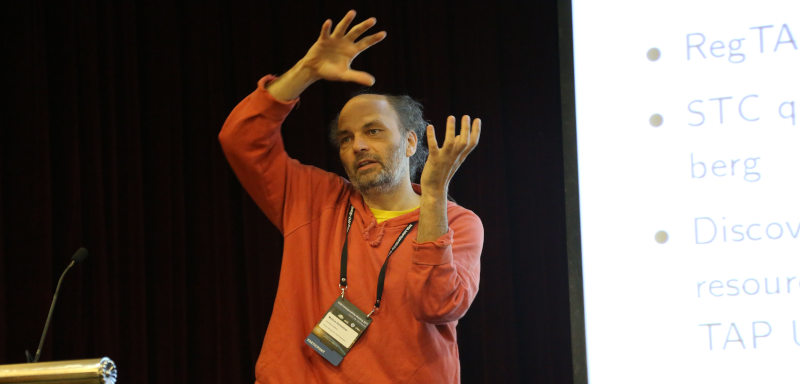
Sometimes, building consensus takes a little bending: Me, at the Shanghai Interop of 2017. In-joke: there's “STC” on the slide.
In the Virtual Observatory, procedures are built on consensus: No (relevant) decisions are passed based some sort of majority vote. While I personally think that's a very good thing in general – you really don't want to clobber minorities, and I couldn't even give a minimal size of such a minority below which it might be ok to ignore them –, there is a profound operational reason for that: We cannot force data centers or software writers to comply with our standards, so they had better agree with them in the first place.
However, building consensus (to avoid Chomsky's somewhat odious notion of manufacturing consent) is hard. In my current work, this insight manifests itself most strongly when I wear my hat as chair of the IVOA Semantics Working Group, where we need to sort items from a certain part of the world into separate boxes and label those, that is, we're building vocabularies. “Part of the world” can be formalised, and there are big phrases like “universe of discourse” to denote such formalisations, but to give you an idea, it's things like reference frames, topics astronomy in general talks about (think journal keywords), relationships between data collections and services, or the roles of files related to or making up a dataset. If you visit the VO's vocabulary repository, you will see what parts we are trying to systematise, and if you skim the current draft for the next release of Vocabularies in the VO, in section two you can find a few reasons why we are bothering to do that.
As you may expect if you have ever tried classifications like this, what boxes (”concepts” in the argot of the semantics folks) there should be and how to label them are questions with plenty of room for dissent. A case study for this is the discussion on VEP-001 and its successors that has been going on since late last year; it also illustrates that we are not talking about bikeshedding here. The discussion clarified much and, in particular, led to substantial improvements not only to the concept in question but also far beyond that. If you are interested, have a look at a few mail threads (here, here, here, or here; more discussion happened live at meetings).
An ideal outcome of such a process is, of course, a solution that is obvious in retrospect, so everyone just agrees. Sometimes, that doesn't happen, and one of these times is VEP-001 and the VEP-003 it evolved into. A spontanous splinter between sessions of this week's Virtual Interop yielded two rather sensible names for the concept we had identified in the previous debates: #sibling on the one hand, and #co-derived on the other (in case you're RDF-minded: the full vocabulary URIs are obtained by prefixing this with the vocabulary URI, http://www.ivoa.net/rdf/datalink/core). Choosing between the two is a bit of a matter of taste, but also of perhaps changing implementations, and so I don't see a clear preference. And the people in the conference didn't reach an agreement before people on the North American west coast really had to have some well-deserved sleep.
In such a situation – extensive discussion yields some very few, apparently rather equivalent solution –, I suspect it is the time to resort to some sort of polling after all. So, in the session I've asked the people involved to give their pain level on a scale of 1 to 10. Given there are quite a few consensus scales out there already (I'm too lazy to look for references now, but I'll retrofit them here if you send some in), I felt this was a bit hasty after I had closed the z**m^H^H^H^H telecon client. But then, thinking about it, I started to like that scale, and so during a little bike ride I came up with what's below. And since I started liking it, I thought I could put it into words, and into a form I can reference when similar situations come up in the future. And so, here it is:
- Oh wow. I'm enthusiastic about it, and I'd get really cross if we didn't do it.
- It's great. I don't think we'll find a better solution. People better have really strong reasons to reject it.
- Fine. Just go ahead.
- Quite reasonable. I have some doubts, but I either don't have a good alternative, or the alternatives certainly won't improve matters.
- Reasonable. I can live with it, possibly accepting a very moderate amount of pain (like: change an implementation that I think is fine as it is).
- Sigh. I don't like it much. If you think it's useful, do it, but don't blame me if it later turns out it stinks.
- Ouch. I wish we didn't have to go there. For instance: This is going to uglify a few things I care about.
- Yikes. I think it's a bad idea. Honestly, let's not do it. It's going to make quite a few things a lot uglier, though I give you it might still just barely work.
- OMG. What are you thinking? I won't go near it, and I pity everyone who will have to. And it's quite likely going to blow up some things I care about.
- Blech. To me, this clearly is a grave mistake that will impact a lot of things very adversely. If I can do anything within reason to stop it, I'll do it. Consider this a veto, and shame on you if you override it.
You can qualify this with:
| +: | I've thought long and hard about this, and I think I understand the matter in depth. You'll hence need arguments of the profundity of the Earth's outer core to sway me. |
|---|---|
| (unqualified): | I've thought about this, and as far as I understand the matter I'm sure about it. More information, solid arguments, or a sudden inspiration while showering might still sway me. |
| -: | This is a gut feeling. It could very well be phantom pain. Feel free to try a differential diagnosis. |
If you like the scale, too, feel free to reference it as href="https://blog.g-vo.org/building-consensus/#scale">https://blog.g-vo.org/building-consensus/#scale.
![[Screenshot: graphs and numbers]](/media/stats_gregory.png)