![[RSS]](../theme/image/rss.png)
Persistent TAP Uploads Update: A Management Interface
There is a new version of the jupyter notebook showing off the persistent TAP uploads in python coming with this post, too: Get it.
Six months ago, I reported on my proposal for persistent uploads into TAP services on this very blog: Basically, you could have and keep your own tables in databases of TAP servers supporting this, either by uploading them or by creating them with an ADQL query. Each such table has a URI; you PUT to it to create it, you GET from it to inspect its metadata, VOSI-style, and you DELETE to it to drop the table once you're done.
Back then, I enumerated a few open issues; two of these I have recently addressed: Lifetime management and index creation. Here is how:
Setting Lifetimes
In my scheme, services assign a lifetime to user-uploaded tables, mainly in order to nicely recover when users don't keep books on what they created. The service will eventually clean up their tables after them, in the case of the reference implementation in DaCHS after a week.
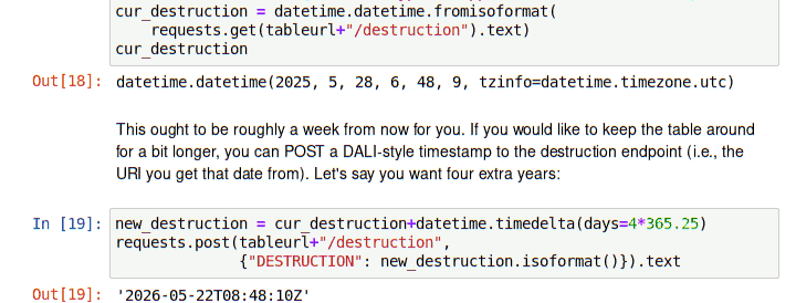
However, there are clearly cases when you would like to extend the lifetime of your table beyond that week. To let users do that, my new interface copies the pattern of UWS. There, jobs have a destruction child. You can post DALI-style timestamps[1] there, and both the POST and the GET return a DALI timestamp of the destruction time actually set; this may be different from what you asked for because services may set hard limits (in my case, a year).
For instance, to find out when the service will drop the table you will create when you follow last October's post you could run:
curl http://dc.g-vo.org/tap/user_tables/my_upload/destruction
To request that the table be preserved until the Epochalypse you would say:
curl -F DESTRUCTION=2038-01-19T03:14:07Z http://dc.g-vo.org/tap/user_tables/my_upload/destruction
Incidentally (and as you can see from the POST response), until January 2037, my service will reduce your request to “a year from now”.
I can't say I'm too wild about posting a parameter called “DESTRUCTION” to an endpoint that's called “destruction” (even if it weren't such a mean word). UWS did that because they wanted it make it easy to operate a compliant service from a web browser. Whether that still is a reasonable design goal (in particular because everyone seems to be wild on dumping 20 metric tons of Javascript on their users even things like UWS would make it easy to not do that) is certainly debatable. But I thought it's better to have a single questionable pattern throughout rather than have something a little odd in one place and something a little less odd in another place.
Creating Indexes
For many applications of database systems, having indexes is crucial. You really, really don't want to have to go through a table with 2 billion rows just to find a single object (that's a quarter of a day when you manage to pull through 100'000 rows a second; ok: today's computers are faster than that). While persistently uploaded tables won't (regularly) have two billion rows any time soon, indexes are already very valuable even for tables in the million-row range.
On the other hand, there are many sorts of indexes, and there are many ways to qualify indexes. To get an idea of what you might want to tell a database about an index, see Postgres' CREATE INDEX docs. And that's just for Postgres; other database systems still do it differently, and of course when you index on expressions, there is no limit to the complexity you can build into your indexes.
Building a cross-database API that would reflect all that is entirely out of the question. Hence, I went for the other extreme: You just specify which column(s) you would like to have indexed, and the service is supposed to choose a plausible index type for you.
Following the model of destruction (typography matters!), this is done by POST-ing one or more column names in INDEX parameters to the index child of the table url. For instance, if you have put a table my_upload that has a column Kmag (e.g., from last October's post), you would say:
curl -L -F INDEX=Kmag http://dc.g-vo.org/tap/user_tables/my_upload/index
The -L makes curl follow the redirect that this issues. Why would it redirect, you ask? The index request creates a UWS job behin the scenes, that is, something like a TAP async job. What you get redirected to is that job.
The background is that for large tables and complex indexes, you may easily get your (appartently idle) connection cut while the index is being created, and you would never learn if a problem had materialised or when the indexing is done. Against that, UWS lets us keep running, and you have a URI at which to inspect the progress of the indexing operation (well, frankly: nothing yet beyond “is it done?”).
Speaking UWS with curl is no fun, but then you don't need to: The job starts in QUEUED and will automatically execute when the machine next has time. In case you are curious, see the notebook linked above, where there is an example for manually following the job's progress. You could use generic UWS clients to watch it, too.
A weak point of the scheme (and one that's surprisingly hard to fix) is that the index is immediately shown in the table metadata the notebook linked to above shows this; I'll spare you the VODataService XML that curl-ing the table URL will spit at you, but in there you will see the Kmag index whether or not the indexer job has run.
It shares this deficit with another way to look at indexes. You see, since there is so much backend-specific stuff you may want to know about an index, I am also proposing that when you GET the index child, you get back the actual database statements, or at least something rather similar. This is expressly not supposed to be machine readable, if only because what you see is highly dependent on the underlying database.
Here is how this looks like on DaCHS over postgres after the index call on Kmag:
$ curl http://dc.g-vo.org/tap/user_tables/my_upload/index
Indexes on table tap_user.my_upload

CREATE INDEX my_upload_Kmag ON tap_user.my_upload (Kmag)
I would not want to claim that this particular human-readable either. But humans that try to understand why a computer does not behave as they expect will certainly appreciate something like this.
Special Index Types
If you look at the tmp.vot from last october's post, you will see that there is an a pair of equatorial coordinates in _RAJ2000 and _DEJ2000. It is nicely marked up with pos.eq UCDs, and the units are deg: This is an example of a column set that DaCHS has special index magic for. Try it:
curl -L -F INDEX=_RAJ2000 -F INDEX=_DEJ2000 \
  http://dc.g-vo.org/tap/user_tables/my_upload/index > /dev/null
Another GET against index will show you that this index is a bit different, stuttering something about q3c (or perhaps spoint at another time or on another service):
Indexes on table tap_user.my_upload

CREATE INDEX my_upload__RAJ2000__DEJ2000 ON tap_user.my_upload (q3c_ang2ipix("_RAJ2000","_DEJ2000"))
CLUSTER my_upload__RAJ2000__DEJ2000 ON tap_user.my_upload
CREATE INDEX my_upload_Kmag ON tap_user.my_upload (Kmag)
DaCHS will also recognise spatial points. Let's quickly create a table with a few points by running:
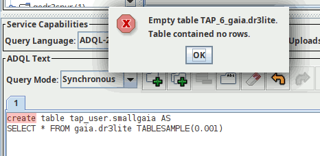
CREATE TABLE tap_user.somepoints AS
SELECT TOP 30 preview, ssa_location
FROM gdr3spec.ssameta
on the TAP server at http://dc.g-vo.org/tap, for instance in TOPCAT (as explained in post one, the “Table contained no rows” message you will see then is to be expected). Since TOPCAT does not know about persistent uploads yet, you have to create the index using curl:
curl -LF INDEX=ssa_location http://dc.g-vo.org/tap/user_tables/somepoints/index
GET-ting the index URL after that will yield:
Indexes on table tap_user.somepoints

CREATE INDEX ndpmaliptmpa_ssa_location ON tap_user.ndpmaliptmpa USING GIST (ssa_location)
CLUSTER ndpmaliptmpa_ssa_location ON tap_user.ndpmaliptmpa
The slightly shocking name of the table is an implementation detail that I might want to hide at some point; the important thing here is the USING GIST that indicates DaCHS has realised that for spatial queries to be able to use the index, a special method is necessary.
Incidentally, I was (and still am) not entirely sure what to do when someone asks for this:
curl -L -F INDEX=_Glon -F INDEX=_DEJ2000 \
  http://dc.g-vo.org/tap/user_tables/my_upload/index > /dev/null
That's a latitude and a longitude all right, but of course they don't belong together. Do I want to treat these as two random columns being indexed together, or do I decide that the user very probably wants to use a very odd coordinate system here?
Well, try it and see how I decided; after this post, you know what to do.
| [1] | Many people call that “ISO format”, but I cannot resist pointing out that ISO, in addition to charging people who want to read their standards an arm and leg, admits a panic-inducing variety of date formats, and so “ISO format” not a particularly useful term. |