Posts with the Tag Astrometry:

  • Making Custom Indexes for astrometry.net

    When you have an image or a scan of a photographic plate, you usually only have a vague idea of what position the telescope actually was pointed at. Furnishing the image with (more or less) precise information about what pixel correesponds to what sky position is called astrometric calibration. For a while now, arguably the simplest option to do astrometric calibration has been a package called astrometry.net. The eponymous web page has been experiencing… um… operational problems lately, but thanks to the Debian astronomy team, there is a nice package for it in Debian.

    However, just running apt install astrometry.net will not give you a working setup. Astrometry.net in addition needs an “index”, files that map star patterns (“quads“, in astrometry.net jargon) to positions. Debian comes with two pre-made sets of indexes at the moment (see apt search astrometry-data): those based on the Tycho 2 catalogue, and those based on 2MASS.

    For the index based on Tycho 2, you will find packages astrometry-data-tycho2-10-19, astrometry-data-tycho2-09, astrometry-data-tycho2-08, astrometry-data-tycho2-07[1]. The numbers in there (“scale numbers”) define the size of images the index is good for: 19 means “a major part of the sky”, 10 is “about a degree”, 8 “about half a degree”. Indexes for large images only have a few bright stars and hence are rather compact, which is why 10 though 19 fit into one package, whereas astrometry-data-tycho2-07-littleendian weighs in at 141 MB, and indexes at scale number 0 (suitable for images of a few arcminutes) take dozens of Gigabytes if they are for the whole sky.

    So, when you do astrometric calibration, consider the size of your images first and then decide which scale number is sensible for you. It is usually a good idea to try the neighbouring scale numbers, too.

    You can then feed these to your calibration routine. If you are running DaCHS, you will probably want to use the AnetHeaderProcessor, where you give the names of the indexes in the sp_indices; you also have to say where to find the indexes, as in:

    from gavo import api
    
    class MyObsCalibrator(api.AnetHeaderProcessor):
      indexPath = "/usr/share/astrometry"
      sp_indices = ["index-tycho2-09*.fits",
        "index-tycho2-10*.fits",
        "index-tycho2-11*.fits",]
    

    This would be suitable for images that cover about a degree on the sky.

    Custom Indexes for Targeted Observations

    The Tycho catalogue starts becoming severely incomplete below mV ≈ 11, and since astrometry.net needs a few stars on an image to be able to calibrate it, you cannot use it to calibrate images smaller than a few tens of arcminutes (depending on where you look, of course). If you have smaller images, there are the 2MASS-based indexes; but the bluer your images are, the worse 2MASS as an infrared survey will do, and in addition, having the giant indexes is a big waste of storage and compute resources when you know your images are on a rather small part of the sky.

    In such a situation, you will save a lot of CPU and possibly even improve your astrometry if you create a custom index for your specific data. For instance, assume you have images sized about 10 arcminutes, and the observation programme covers a reasonably small set of objects (as long as it's of order a few hundred, a custom index certainly will be a good deal). You could then make your index based on Gaia positions and photometry like this:

    """
    Create an index for astrometry.net and a few small fields based on Gaia.
    
    Be sure to adapt this for your use case; for instance, if what your are
    calibrating will be from only a part of the sky, pick specific healpixes
    (perhaps on a different level; below, we're using level 5).  Also consider
    changing the target epoch, the photometry, or the magnitude limit.
    
    This script takes the sample positions from a text file; have
    space-separated pairs of ra and dec in targets.txt.
    """
    
    import os
    import subprocess
    
    from astropy.table import Table
    import pyvo
    
    # 0 is for images of about two arcminutes, 10 for about degree, 12 for two
    # degrees, etc.
    SIZE_PRESET = 1
    
    # The typical radius of your images in degrees (this is the size of our cone
    # searches, so cut some slack); this needs to be changed in unison with
    # SIZE_PRESET
    IMAGE_RADIUS = 1/10.
    
    
    def get_target_table():
        """must return an astropy table with columns ra and dec in degrees.
    
        (of course, if you have your data in a proper format with actual metadata,
        you don't need any of the ugly magic).
        """
        targets = Table.read("targets.txt", format="ascii")
        targets["col1"].name, targets["col2"].name = "ra", "dec"
        targets["ra"].meta = {"ucd": "pos.eq.ra;meta.main"}
        targets["dec"].meta = {"ucd": "pos.eq.dec;meta.main"}
        return targets
    
    
    def main():
        tap_service = pyvo.dal.TAPService("http://dc.g-vo.org/tap")
        res = tap_service.run_async(f"""
            SELECT g.ra as RA, g.dec as DEC, phot_g_mean_mag as MAG
            FROM gaia.dr3lite AS g
            JOIN TAP_UPLOAD.t1 as mine
                ON DISTANCE(mine.ra, mine.dec, g.ra, g.dec)<{IMAGE_RADIUS}""",
          uploads={"t1": get_target_table()})
    
        cat_file = "basic-cat.fits"
        res.to_table().write(cat_file, format="fits", overwrite=True)
    
        try:
            subprocess.run(["build-astrometry-index", "-i", cat_file,
                "-o", f"./index-custom-{SIZE_PRESET:02d}.fits",
                "-P", str(SIZE_PRESET), "-S", "MAG"])
        finally:
            os.unlink(cat_file)
    
    
    if __name__=="__main__":
        main()
    

    This writes a single file, index-custom-01.fits (in this case).

    If you read your positions from something else than the simple ASCII file I'm assuming here: Be sure to annotate the columns containing RA and Dec with the proper UCDs as shown here. That makes DaCHS (and perhaps other TAP services, too) create the right hints for the database, speeding up things tremendously.

    You can of course change the ADQL query; it might, for instance, help to replace the G magnitudes with RP or BP ones, or you could use a different catalogue than Gaia. Just make sure the FITS table that is written to basic-cat.fits has exactly the columns RA, DEC, and MAG.

    In DaCHS, I tend to keep scripts like the one above in a subdirectory of the resdir called custom-index, and then in the calibration script I write:

    from gavo import api
    
    RD = api.getRD("myres/q")
    
    class MyObsCalibrator(api.AnetHeaderProcessor):
      indexPath = RD.resdir
      sp_indices = ["custom-index/index-custom-01.fits"]
    

    Custom Indexes for Ancient Observations

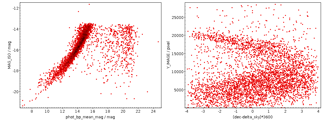
    On the other hand, if you have oldish images not going terribly deep, you may want to tailor an index for about the epoch the images were taken at. Many bright stars have a proper motion large enough to matter over a century, and so doing epoch propagation (in this case with the ivo_epoch_prop user defined function, which is not available everywhere) is probably a good idea. The following script computes three full-sky indexes with quads around the desired size; note how you can set the limiting magnitude and the size preset:

    """
    Create a full-sky index for bright stars and astrometry.net based on Gaia.
    
    This only works for rather bright stars because the Gaia service will refuse
    to server more than ~1e7 objects.
    
    Make sure to choose SIZE_PRESET to your use case (19 means 30 deg,
    10 about a degree, two preset steps are about a factor two in scale).
    """
    
    import os
    import subprocess
    
    import pyvo
    
    # see the module docstring
    SIZE_PRESET = 12
    
    # ignore stars fainter than this; you can't go below 14 all-sky with Gaia
    # and the GAVO DC server
    MAX_MAG = 12
    
    # Epoch to transform the stars to
    TARGET_EPOCH = 1910
    
    
    def main():
        tap_service = pyvo.dal.TAPService("http://dc.g-vo.org/tap")
        res = tap_service.run_async(f"""
            SELECT pos[1] as RA, pos[2] as DEC, mag as MAG
            FROM (
                SELECT phot_bp_mean_mag AS mag,
                    ivo_epoch_prop(ra, dec, parallax,
                        pmra, pmdec, radial_velocity, 2016, {TARGET_EPOCH}) as pos
                FROM gaia.dr3lite
              WHERE phot_bp_mean_mag<{MAX_MAG}) AS q""")
    
        cat_file = "current.fits"
        res.to_table().write(cat_file, format="fits", overwrite=True)
    
        try:
            for size_preset in range(SIZE_PRESET-1, SIZE_PRESET+2):
                subprocess.run(["build-astrometry-index", "-i", cat_file,
                    "-o", f"./index-custom-{size_preset:02d}.fits",
                    "-P", str(size_preset), "-S", "MAG"])
        finally:
            os.unlink(cat_file)
    
    
    if __name__=="__main__":
        main()
    

    With this and my custom-index directory, your DaCHS header processor could say:

    from gavo import api
    
    RD = api.getRD("myres/q")
    
    class MyObsCalibrator(api.AnetHeaderProcessor):
      indexPath = RD.resdir
      sp_indices = ["custom-index/index-custom-*.fits"]
    

    Custom Indexes: Full-sky and Deep

    I have covered the cases “deep and spotty” and “shallow and full-sky“. The case “deep and full-sky“ is a bit more involved because it still lies in the realm of big data, which always requires extra tricks. In this case, that would be retrieving the basic catalogue in parts – for instance, by HEALPix – and at the same time splitting the index up between HEALPixes, too. This does not require great magic, but it does require a bit of non-trivial bookkeeping, and hence I will only write about it if someone actually needs it – if that's you, please write in.

    [1]You will also find that each of these exist in a littleendian and bigendian flavours; ignore these, your machine will pick what it needs when you install the packages without tags.
  • Computing Residuals of an Astrometric Calibration

    Two plots, left a fairly good correlation, right a cloudy wave

    The kind of plot you can make following the recipe given here: Left, a comparison of the photometry, right, a positional residuals, not taking into account the SIP plate solution, when comparing the HDAP plate B3261a against Gaia DR3. Note that the cut-off a 4 arcsec is because of the match radius when obtaining the calibrator stars.

    I recently had to assess the quality of the astrometric calibration of a photographic plate. What I am going to show you in this post will of course work just as well for CCD frames, and if these have a sufficiently large field of view, this may be an issue for them as well. However, the sort of data that needs this assessment most typically are scans of plates, as these tend to have a “wobble”, systematic offsets in the scan direction resulting from imperfections in the mechanics.

    Prerequisites: An astronomical frame with a calibration in ICRS (or some frame not very far from it), called my-image.fits in the following, SExtractor (in Debian and derivatives: apt install source-extractor – long live Debian Astro; since it's called source-extractor in Debian, that's what I'll use here, too), and of course TOPCAT.

    Step 1: Extract Sources. Source extraction is of course a high science, and if you know better than me, by all means do it the way you think is appropriate. Meanwhile, the following might very well work for you sufficiently well.

    Create a working directory and enter it. Then, to create a file telling source-extractor what columns you would like to see, write the following to a file default.param:

    ALPHA_SKY
    DELTA_SKY
    X_IMAGE
    Y_IMAGE
    MAG_ISO
    FLUX_AUTO
    ELONGATION
    

    Next, give a few parameters to source-extractor; depending on the sort of image you have, you may want to play around with DETECT_MINAREA (how many pixels need to show a signal to register as a source) and DETECT_THRESH (how many sigmas a pixel has to be above the background to register as a candidate for belonging to a source). Meanwhile, write the following into a file default.control:

    CATALOG_TYPE     FITS_1.0
    CATALOG_NAME     img.axy
    PARAMETERS_NAME  default.param
    FILTER           N
    DETECT_MINAREA   30
    DETECT_THRESH    4
    SEEING_FWHM      1.2
    

    – but if the following call gives you a few hundred sources, that ought to work for the present purpose.

    Then run:

    source-extractor -c default.control my-image.fits
    

    This will give you a catalogue of extracted objects in the file img.axy.

    Step 2: Fix source-extractor's output. Load that img.axy into TOPCAT. Regrettably, source-extractor does not add any useful metadata to the columns of its output table. To add the absolute bare minimum, in TOPCAT go to ViewsColumn Info. In that window, check UCD in the Display menu, and then put pos.eq.ra and pos.eq.dec into the UCD fields of the ALPHA_SKY and DELTA_SKY columns, respectively; double click to change fields in TOPCAT.

    To see if you have done the annotation right, in TOPCAT's main window, click GraphicsSky Plot. If the objects show up, you have just provided enough annotation to let TOPCAT figure out the position for each row.

    Step 3: Get calibrators. We will now try to add counterparts for Gaia DR3 to the extracted sources. To do that, click VOTable Access Protocol, and in the window popping up double click the entry for the GAVO DC TAP.

    In the Find box, type dr3lite to look for this site's version of the Gaia DR3 source catalogue. Click on gaia.dr3lite to select that table, and then select the Columns pane. This should show some of the Gaia DR3 columns.

    Now ExamplesUpload Join will generate a query that will cross-match your extracted sources with the Gaia sources. You should edit it a bit, only selecting the columns you will actually need, removing the TOP 1000 (at least on large images with more than 1000 sources), and reducing the match radius a bit when the calibration is not actually completely off and your epoch is sufficiently close to J2000.

    Hint: you can control-click in the Columns pane and then use the Cols button to insert all the column names in one go[1]. For me, the resulting query would be:

    SELECT
       source_id, ra, dec, phot_bp_mean_mag,
       tc.*
       FROM gaia.dr3lite AS db
       JOIN TAP_UPLOAD.t1 AS tc
       ON 1=CONTAINS(POINT('ICRS', db.ra, db.dec),
                     CIRCLE('ICRS', tc.ALPHA_SKY, tc.DELTA_SKY, 4./3600.))
    

    This should result in about as many matches as your extraction had – a few more is ok, because you will have some spurious matches, a few less is ok, too, as there are always some outliers and artefacts, but you should clearly not pull a magnitude more or less objects here than you put in; fiddle with the match radius as necessary.

    See if there is a rough correlation between the Gaia calibrators and your extracted sources by plotting phot_bp_mean_mag against MAG_ISO. Absent more information, MAG_ISO, source-extractor's guess for the magnitude of the extracted object, will be just some crazy number, but it should have some discernable correlation with the actual magnitude. Do not expect too much here, in particular with old plates, for which good photometry is a science of their own.

    In my example, this looked like this:

    Plot: a rough correlation in red with a green tail

    The green points certainly are spurious matches; this observation did not reach beyond 14th magnitude or so, and there are many weak stars on the sky, so a few of them will show up in just about any cross match. See the opening picture for an example with a better correlation.

    Step 4: Do the correlation plot. Do GraphicsPlane Plot and then plot ra-alpha_sky or dec-delta_sky against X_IMAGE or Y_IMAGE. You could get something like this:

    Plot: A single wavy thing

    This rather certainly reflects some optical distortion; source-extractor regrettably does not take into account SIP corrections yet, so it is likely that a large part of this would be taken care of by the polynomials of the plate solution (the github issue I am linking to tells you how to be sure).

    But it can also look like this:

    Plot: Multiple wobbles

    This certainly is not the result of a lens or anything optical at all. It's the scanner's gears that you are looking at here. With an amplitude of perhaps three arcseconds this is rather excessive here; but something like this you will rather likely see even on good scanners – though it may essentially be invisible, as of the Heidelberg scanner we used for HDAP:

    Plot: A vertical cloud with no discernible structure.
    [1]I'm using the BP magnitude in the query below as most historical plates tend to be “blue sensitive“ (in some sense). Hence, BP magnitudes should be a bit closer to what source-extractor has extracted.
  • The Loneliest Star in the Sky

    sky images and a distribution plot

    The loneliest star in the sky on the left, and on the right a somewhat more lonelier one (it's explained in the text). The inset shows the distribution of the 500 loneliest stars on the whole sky in Galactic coordinates.

    In early December, the object catalogue of Gaia's data release 3 was published (“eDR3“), and I've been busy in various ways on this data off and on since then – see, for instance, the The Case of the disappearing bits on this blog.

    One of the things I have missed when advising people on projects with previous Gaia data releases is a table that, for every object, gives the nearest neighbour. And so for this release I've created it and christened it, perhaps just a bit over-grandiosely, “Gaia eDR3 Autocorrelation”. Technically, it is just a long (1811709771 rows, to be precise) list of pairs of Gaia eDR3 source ids, the ids of their nearest neighbour, and a spherical distance between.

    This kind of data is useful for many applications, mostly when looking for objects that are close together or (more often) things that fail for such close pairs for a wide variety of reasons. I have taken some pains to not only have close neighbours, though, because sometimes you may want specifically objects far away from others.

    As in the case of this article's featured image: The loneliest star in the sky (as seen by Gaia, that is) is eDR3 6049144983226879232, which is 4.3 arcminutes from its neighbour, 6049144021153793024, which in turn is the second-loneliest star in the sky. They are, perhaps a bit surprisingly, in Ophiuchus (and thus fairly close to the Milky Way plane), and (probably) only about 150 parsec from Earth. Doesn't sound too lonely, hm? Turns out: these stars are lonely because dust clouds blot out all their neighbours.

    Rank three is in another dust cloud, this time in Taurus, and so it continues in low Galactic latitude to rank 8 (4402975278134691456) at Galactic latitude 36.79 degrees; visualising the thing, it turns out it's again in a dark cloud. What about rank 23 at 83.92 Galactic (3954600105683842048)? That's probably bona-fide, or at least it doesn't look very dusty in the either DSS or PanSTARRS. Coryn (see below) estimates it's about 1100 parsec away. More than 1 kpc above the galactic disk: that's more what I had expected for lonely stars.

    Looking at the whole distribution of the 500 loneliest stars (inset above), things return a bit more to what I had expected: Most of them are around the galactic poles, where the stellar density is low.

    So: How did I find these objects? Here's the ADQL query I've used:

    SELECT TOP 500
      ra, dec, source_id, phot_g_mean_mag, ruwe,
      r_med_photogeo,
      partner_id, dist,
      COORD2(gavo_transform('ICRS', 'GALACTIC',
        point(ra, dec))) AS glat
    FROM
      gedr3dist.litewithdist
      NATURAL JOIN gedr3auto.main
    ORDER BY dist DESC
    

    – run this on the TAP server at http://dc.g-vo.org/tap (don't be shy, it's a cheap query).

    Most of this should be familiar to you if you've worked through the first pages of ADQL course. There's two ADQL things I'd like to advertise while I have your attention:

    1. NATURAL JOIN is like a JOIN USING, except that the database auto-selects what column(s) to join on by matching the columns that have the same name. This is a convenient way to join tables designed to be joined (as they are here). And it probably won't work at all if the tables haven't been designed for that.
    2. The messy stuff with GALACTIC in it. Coordinate transformations had a bad start in ADQL; the original designers hoped they could hide much of this; and it's rarely a good idea in science tools to hide complexity essentially everyone has to deal with. To get back on track in this field, DaCHS servers since about version 1.4 have been offering a user defined function gavo_transfrom that can transform (within reason) between a number of popular reference frames. You will find more on it in the server's capabilities (in TOPCAT: the “service” tab). What is happening in the query is: I'm making a Point out of the RA and Dec given in the catalogue, tell the transform function it's in ICRS and ask it to make Galactic coordinates from it, and then take the second element of the result: the latitude.

    And what about the gedr3dist.litewithdist table? That doesn't look a lot like the gaiaedr3.gaiasource we're supposed to query for eDR3?

    Well, as for DR2, I'm again only carrying a “lite” version of the Gaia catalogue in GAVO's Heidelberg data center, stripped down to the columns you absolutely cannot live without even for the most gung-ho science; it's called gaia.edr3lite.

    But then my impression is that almost everyone wants distances and then hacks something to make Gaia's parallax work for them. That's a bad idea as the SNR goes down to levels very common in the Gaia result catalogue (see 2020arXiv201205220B if you don't take my word for it). Hence, I'm offering a pre-joined view (a virtual table, if you will) with the carefully estimated distances from Coryn Bailer-Jones, and that's this gedr3dist.litewithdist. Whenever you're doing something with eDR3 and distances, this is where I'd point you first.

    Oh, and I should be mentioning that, of course, I figured out what is in dust clouds and what is not with TOPCAT and Aladin as in our tutorial TOPCAT and Aladin working together (which needs a bit of an update, but you'll figure it out).

    There's a lot more fun to be had with this (depending on what you find fun in). What about finding the 10 arcsec-pairs with the least different luminosities (which might actually be useful for testing some optics)? Try this:

    SELECT TOP 300
      a.source_id, partner_id, dist,
      a.phot_g_mean_mag AS source_mag,
      b.phot_g_mean_mag AS partner_mag,
      abs(a.phot_g_mean_mag-b.phot_g_mean_mag) AS magdiff
    FROM gedr3auto.main
      NATURAL JOIN gaia.edr3lite AS a
      JOIN gaia.edr3lite AS b
        ON (partner_id=b.source_id)
    WHERE
      dist BETWEEN 9.999/3600 AND 10.001/3600
      AND a.phot_g_mean_mag IS NOT NULL
      AND b.phot_g_mean_mag IS NOT NULL
    ORDER BY magdiff ASC
    

    – this one takes a bit longer, as there's many 10 arcsec-pairs in eDR3; the query above looks at 84690 of them. Of course, this only returns really faint pairs, and given the errors stars that weak have they're probably not all that equal-luminosity as that. But fixing all that is left as an exercise to the reader. Given there's the RP and BP magnitude columns, what about looking for the most colourful pair with a given separation?

    Acknowledgement: I couldn't have coolly mumbled about Ophiuchus or Taurus without the SCS service ivo://cds.vizier/vi/42 (”Identification of a Constellation From Position, Roman 1982”).

    Update [2021-02-05]: I discovered an extra twist to this story: Voyager 1 is currently flying towards Ophiuchus (or so Wikipedia claims). With an industrial size package of artistic licence you could say: It's coming to keep the loneliest star company. But of course: by the time Voyager will be 150 pc from earth, eDR3 6049144983226879232 will quite certainly have left Ophiuchus (and Voyager will be in a completely different part of our sky, that wouldn't look familar to us at all) – so, I'm afraid apart from a nice conincidence in this very moment (galactically speaking), this whole thing won't be Hollywood material.

  • See Who's Kinking the Sky

    A new arrival in the GAVO Data Center is UCAC5, another example of a slew of new catalogs combining pre-existing astrometry with Gaia DR1, just like the HSOY catalog we've featured here a couple of weeks back.

    That's a nice opportunity to show how to use ADQL's JOIN operator for something else than the well-known CONTAINS-type crossmatch. Since both UCAC5 and HSOY reference Gaia DR1, both have, for each object, a notion which element of the Gaia source catalog they correspond to. For HSOY, that's the gaia_id column, in UCAC5, it's just source_id. Hence, to compare results from both efforts, all you have to do is to join on source_id=gaia_id (you can save yourself the explicit table references here because the column names are unique to each table.

    So, if you want to compare proper motions, all you need to do is to point your favourite TAP client's interface to http://dc.g-vo.org/tap and run:

    SELECT
        in_unit(avg(uc.pmra-hsoy.pmra), 'mas/yr') AS pmradiff,
        in_unit(avg(uc.pmde-hsoy.pmde), 'mas/yr') AS pmdediff,
        count(*) as n,
        ivo_healpix_index (6, raj2000, dej2000) AS hpx
        FROM hsoy.main AS hsoy
        JOIN ucac5.main as uc
        ON (uc.source_id=hsoy.gaia_id)
        WHERE comp IS NULL    -- hsoy junk filter
        AND clone IS NULL     -- again, hsoy junk filter
        GROUP BY hpx
    

    (see Taylor et al's All of the Sky if you're unsure what do make of the healpix/GROUP BY magic).

    Of course, the fact that both tables are in the same service helps, but with a bit of upload magic you could do about the same analysis across TAP services.

    Just so there's a colourful image in this post, too, here's what this query shows for the differences in proper motion in RA:

    (equatorial coordinates, and the aux axis is a bit cropped here; try for yourself to see how things look for PM in declination or when plotted in galactic coordinates).

    What does this image mean? Well, it means that probably both UCAC5 and HSOY would still putt kinks into the sky if you wait long enough.

    In the brightest and darkest points, if you waited 250 years, the coordinate system induced by each catalog on the sky would be off by 1 arcsec with respect to the other (on a sphere, that means there's kinks somewhere). It may seem amazing that there's agreement to at least this level between the two catalogs – mind you, 1 arcsec is still more than 100 times smaller than you could see by eye; you'd have to go back to the Mesolithic age to have the slightest chance of spotting the disagreement without serious optical aids. But when Gaia DR2 will come around (hopefully around April 2018), our sky will be more stable even than that.

    Of course, both UCAC5 and HSOY are, indirectly, standing on the shoulders of the same giant, namely Hipparcos and Tycho, so the agreement may be less surprising, and we strongly suspect that a similar image will look a whole lot less pleasant when Gaia has straightened out the sky, in particular towards weaker stars.

    But still: do you want to bet if UCAC5 or HSOY will turn out to be closer to a non-kinking sky? Let us know. Qualifications („For bright stars...”) are allowed.

Page 1 / 1