Articles from Data

• A Data Publisher's Diary: Wide Images in DASCH

  2024-05-03 Markus Demleitner

  

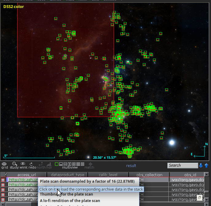
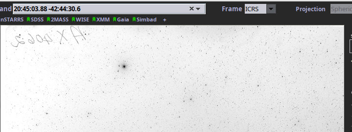
  This is the new resonse when you query the DASCH SIAP service for Aladin's default view on the horsehead nebula. As you can see, at least the returned images no longer are distributed over half of the sky (note the size of the view).

  The first reaction I got when the new DASCH in the VO service hit Aladin was: “your SIAP service is broken, it just dumps all images it has at me rather than honouring my positional constraint.”

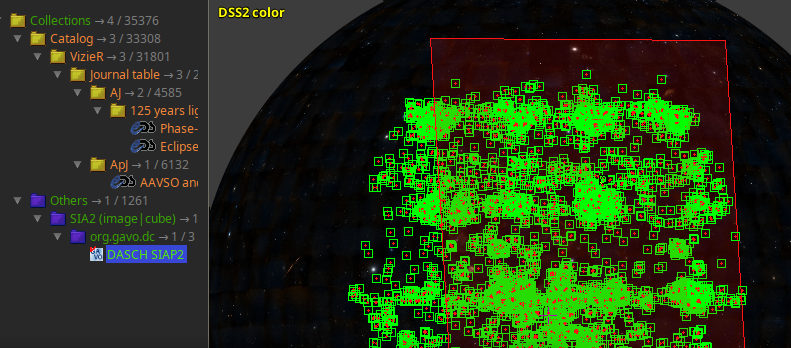
  I have to admit I was intially confused as well when an in-view search from Aladin came back with images with centres on almost half the sky as shown in my DASCH-in-Aladin illustration. But no, the computer did the right thing. The matching images in fact did have pixels in the field of view. They were just really wide field exposures, made to “patrol” large parts of the sky or to count meteors.

  DASCH's own web interface keeps these plates out of the casual users' views, too. I am following this example now by having two tables, dasch.narrow_plates (the “narrow” here follows DASCH's nomenclature; of course, most plates in there would still count as wide-field in most other contexts) and dasch.wide_plates. And because the wide plates are probably not very helpful to modern mainstream astronomers, only the narrow plates are searched by the SIAP2 service, and only they are included with obscore.

  In addition to giving you a little glimpse into the decisions one has to make when running a data centre, I wrote this post because making a provisional (in the end, I will follow DASCH's classification, of course) split betwenn “wide” and “narrow” plates involved a bit of simple ADQL that may still be not totally obvious and hence may merit a few words.

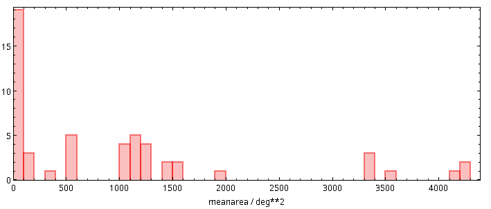
  My first realisation was that the problem is less one of pixel scale (it might also be) but of the large coverage. How do we figure out the coverage of the various instruments? Well, to be robust against errors in the astrometric calibration (these happen), let us average; and average over the area of the polygon we have in s_region, for which there is a convenient ADQL function. That is:

  SELECT instrument_name, avg(area(s_region)) as meanarea
  FROM dasch.plates
  GROUP BY instrument_name
  

  It is the power of ADQL aggregate function that for this characterisation of the data, you only need to download a few kilobytes, the equivalent of the following histogram and table:

  

  Instrument Name	mean size [sqdeg]
  Eastman Aero-Ektar K-24 Lens on a K-1...
  Cerro Tololo 4 meter
  Logbook Only. Pages without plates.
  Roe 6-inch
  Palomar Sky Survey (POSS)
  1.5 inch Ross (short focus)	4284.199799877725
  Patrol cameras	4220.802442888225
  1.5-inch Ross-Xpress	4198.678060743206
  2.8-inch Kodak Aero-Ektar	3520.3257323233624
  KE Camera with Installed Rough Focus	3387.5206396388453
  Eastman Aero-Ektar K-24 Lens on a K-1...	3370.5283986677637
  Eastman Aero-Ektar K-24 Lens on a K-1...	3365.539790633015
  3 inch Perkin-Zeiss Lens	1966.1600884072298
  3 inch Ross-Tessar Lens	1529.7113188540836
  2.6-inch Zeiss-Tessar	1516.7996790591587
  Air Force Camera	1420.6928219265849
  K-19 Air Force Camera	1414.074101143854
  1.5 in Cooke "Long Focus"	1220.3028263587332
  1 in Cook Lens #832 Series renamed fr...	1215.1434235932702
  1-inch	1209.8102811770807
  1.5-inch Cooke Lenses	1209.7721123964636
  2.5 inch Cooke Lens	1160.1641223648048
  2.5-inch Ross Portrait Lens	1137.0908812243645
  Damons South Yellow	1106.5016573891376
  Damons South Red	1103.327982978934
  Damons North Red	1101.8455616455205
  Damons North Blue	1093.8380971825375
  Damons North Yellow	1092.9407550755682
  New Cooke Lens	1087.918570304363
  Damons South Blue	1081.7800084709982
  2.5 inch Voigtlander (Little Bache or...	548.7147592220762
  NULL	534.9269386355818
  3-inch Ross Fecker	529.9219051692568
  3-inch Ross	506.6278856912204
  3-inch Elmer Ross	503.7932693652602
  4-inch Ross Lundin	310.7279860552893
  4-inch Cooke (1-327)	132.690621660727
  4-inch Cooke Lens	129.39637516917298
  8-inch Bache Doublet	113.96821604869973
  10-inch Metcalf Triplet	99.24964308212328
  4-inch Voightlander Lens	98.07368690379751
  8-inch Draper Doublet	94.57937153909593
  8-inch Ross Lundin	94.5685388440282
  8-inch Brashear Lens	37.40061588712761
  16-inch Metcalf Doublet (Refigured af...	33.61565584978583
  24-33 in Jewett Schmidt	32.95324914757339
  Asiago Observatory 92/67 cm Schmidt	32.71623733985344
  12-inch Metcalf Doublet	31.35112644688316
  24-inch Bruce Doublet	22.10390937657793
  7.5-inch Cooke/Clark Refractor at Mar...	14.625992810622787
  Positives	12.600189007151709
  YSO Double Astrograph	10.770798601877804
  32-36 inch BakerSchmidt 10 1/2 inch r...	10.675406541122827
  13-inch Boyden Refractor	6.409447066606171
  11-inch Draper Refractor	5.134521254785461
  24-inch Clark Reflector	3.191361603405415
  Lowel 40 inch reflector	1.213284257086087
  200 inch Hale Telescope	0.18792105301170514

  For the instruments with an empty mean size, no astrometric calibrations have been created yet. To get a feeling for what these numbers mean, recall that the celestial sphere has an area of 4 π rad², that is, 4⋅180²/π or 42'000 square degrees. So, some instruments here indeed covered 20% of the night sky in one go.

  I was undecided between cutting at 150 (there is a fairly pronounced gap there) or at 50 (the gap there is even more pronounced) square degrees and provisionally went for 150 (note that this might still change in the coming days), mainly because of the distribution of the plates.

  You see, the histogram above is about instruments. To assess the consequences of choosing one cut or the other, I would like to know how many images a given cut will remove from our SIAP and ObsTAP services. Well, aggregate functions to the rescue again:

  SELECT ROUND(AREA(s_region)/100)*100 AS platebin, count(*) AS ct
  FROM dasch.plates
  GROUP BY platebin
  

  To plot such a pre-computed histogram in TOPCAT, tell the histogram plot window to use ct as the weight, and you will see something like this:

  

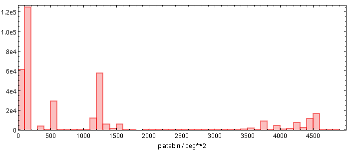
  It was this histogram that made me pick 150 deg² as the cutoff point for what should be discoverable in all-VO queries: I simply wanted to retain the plates in the second bar from left.

• DASCH is now in the VO

  2024-04-29 Markus Demleitner

  

  This frame would show comet 2P/Encke during its proximity to Earth in 1941 – if it went deep enough. But never mind practicalities: If you want to learn about matching ephemeris against the DASCH plate collection (or, really, any sort of obscore-like table), read on.

  • Why Bother?
  • DASCH: The Harvard Plates
  • Plates in Global Discovery
  • TAP, Uploads, and pyVO on DASCH
  • Disclaimers

  For about a century – that is, into the 1980s –, being an observational astronomer meant taking photographic plates and doing tricks with them (unless you were a radio astronomer or one of the very few astronomers peeking beyond radio and optical in those days, of course). This actually is somewhat fortunate for archivists, because unlike many of the early CCD observations that by now are lost with our ability to read the tapes they were stored on, the plates are still there.

  Why Bother?

  However, to make them usable, the plates need to be digitised. In the GAVO data centre, we keep the results of several scan campaigns large and small, such as HDAP, the various data collections joined in the historical photographic plate image archive HPPA, or the delightfully quirky Münster Flare Plates.

  I personally care a lot about these data collections. This is partly because they are indispensible for understanding the history of astronomy. But more importantly, they are the next best thing we have to a time machine; if we have a way of knowing how the sky looked like seventy years ago, it is these plate collections. Having such a time machine is important for all kinds of scientific efforts, including figuring out whether there are aliens (i.e., 2016ApJ...822L..34S) on Tabby's Star.

  Somewhat to my chagrin, the cited paper 2016ApJ...822L..34S did not use the VO to obtain the plate images but went straight to DASCH's web interface. DASCH, in case you have not heard of it before, is probably the most ambitious project concerned with plate digitisation at the moment – or perhaps: “was”, because they just finished scanning the core part of Harvard's plate collections, which was their primary goal.

  I can understand why Bradley Schaefer, the paper's author, did not bother with a VO search In 2016. For starters, working with halfway homogeneous data from instruments you are somewhat familiar saves a substantial amount of work and thought, in particular if you are, in addition, up against the usual lack of machine-readable metadata. Also, at that time DASCH probably had about as many digitised plates as all the VO's contemporary plate collections taken together.

  DASCH: The Harvard Plates

  Given such stats, I have always wanted to have at least the metadata from DASCH's plates in the VO. Thanks to a recent update to DASCH's publication system, this is now a reality. Since 2024-04-29, I am publishing the metadata of the DASCH plates via Obscore and and SIAP2.

  Followup (2024-05-03)

  This is now DASCH news, and one of my two main contacts on the DASCH side, Peter Williams, has written an insightful post on this, too. Let me use this opportunity to thank him for the delightful cooperation, and extend these thanks to Ben Sabath, who is primarily responsible for the update to the DASCH publication system I mentioned above.

  Matching plates are returned as datalink documents, pointing to a preview, photos of the plate and its jacket, and links to the science data, once downsampled by a factor of 16, once in the original size (example). For now, #this points to the downsampled version, as Amazon charges DASCH about three cents per full-scale plate at the moment, and that can quickly add up by accident (there's nothing wrong with consciously downloading full-scale FITS-es if you need them, of course).

  This is a bit fishy in that the size of the image in the obscore/SIAP2 fields s_xel1 and s_xel2 refers to the unscaled image, and thus I should be returning the full-scale image as datalink #this. I hope I will not cause much confusion with this design.

  In case you look at the links in the datalink documents, let me include a disclaimer: Although they point into the GAVO data centre, the data is served courtesy of the DASCH project. The links only go to us because we need to sign links for you. I mention this because you can save the datalink documents and the links within them; the URLs you are redirected to from there, however, will expire fast. Just do not look at them.

  Plates in Global Discovery

  So – what can you do with DASCH in the VO that you could not do before?

  Most importantly, you will discover DASCH in registry interfaces and its datasets in global queries (in particular the global dataset queries I have discussed a few weeks ago). For instance, DASCH is now in Aladin's discovery tree:

  

  You can now find DASCH in Aladin and do the usual “in view“ searches. However, currently this yields many matches that are, in practical terms, spurious, as they come from extremely wide-angle instruments. The red rectangle is the footprint of one of these images; note that the view here is a full two pi sky. We will probably do something about this “noise“.

  The addition of DASCH to the VO has a strong effect in some use cases. For instance, at the end of the GAVO plates tutorial, we do an all-VO obscore query that, at the time of the last update of the tutorial in 2019, yielded 4067 datasets (of course, including modern and/or non-optical observations) potentially showing some strongly lensed quasar. With DASCH – and, admittedly, a few more collections that came into the VO since 2019 –, that number is now 10'489; the range of observation dates grew from MJD 12550…52000 to MJD 9800…58600, with the mean decreasing from 51'909 to 30'603. That the mean observation date moves that much back in time is a certain sign that a major part of the expansion is due to DASCH (well, and certainly to APPLAUSE, too).

  Followup (2024-05-03)

  As discussed in my DASCH update, I have taken out the large-coverage plates from my obscore table, which changes the stats (but not the conclusions) quite a bit. They is now 10'098 plates and mean observation date 36'396

  TAP, Uploads, and pyVO on DASCH

  But this is not just about bringing astronomical heritage to the VO. It is also about exposing DASCH through the powerful ADQL/TAP interface. As an example of how this may be useful, consider the comet P2/Encke, which, according to JPL's Small-Body Database was relatively close to Earth (about half an AU) in May 1941. It would have had about 14.5 mag at that point and hence was safely within reach of several of the instruments archived in DASCH. Perhaps we can find serendipitous or even targeted observations of the comet in the collection?

  The plan to find that out is: compute an ephemeris (we are lazy and use an external service, Miriade ephemcc) and then for each day see whether there are DASCH observations in the vicinity of the sky location obtained in this way.

  As usual, it's never that easy because the call to the ephemeris webservice (paste the link into TOPCAT to have a look) returns cursed sexagesimal coordinates. We need to fix them before doing anything serious with the table, and while we are at it, we also repair the date, which is simpler to consume if it is MJD to begin with. Getting the ephemeris thus takes quite a few lines:

  from astropy import table
  from astropy import units as u
  from astropy.coordinates import SkyCoord
  from astropy.time import Time
  
  ephem = table.Table.read(
    "https://vo.imcce.fr/webservices/miriade/ephemcc.php?-from=vespa"
    "&-name=c:p/encke&-ep=1941-04-01&-nbd=90&-step=1d&-observer=500"
    &-mime=votable")
  
  parsed = SkyCoord(ephem["ra"], ephem["dec"], unit=(u.hourangle, u.deg))
  ephem["ra"] = parsed.ra.degree
  ephem["dec"] = parsed.dec.degree
  
  parsed = Time(ephem["epoch"])
  ephem["epoch"] = parsed.mjd
  

  Compared to that, the actual matching against DASCH is almost trivial if you are somewhat familiar with crossmatching in ADQL and the Obscore schema:

  svc = pyvo.dal.TAPService("http://dc.g-vo.org/tap")
  res = svc.run_sync("""
      SELECT *
      FROM
          dasch.plates
          JOIN tap_upload.orbit
          ON (1=CONTAINS(POINT(ra, dec), s_region))
      WHERE
          t_min<epoch
          AND t_max>epoch""",
      uploads={"orbit": ephem})
  

  Followup (2024-05-03)

  You would probably query the dasch.narrow_plates table in actual operations; querying dasch.plates is probably more for people interested in the history of astronomy or DASCH itself.

  Inspect the query for a moment: This is a normal upload join, except we are constructing an ADQL POINT on the fly to be able to see whether we are in the spatial region covered by a DASCH dataset (given in obscore's s_region column). We could have put the temporal condition into the join's ON; but I think the intention is somewhat clearer with the WHERE constraint, and the database engine will probably go through identical motions for both queries – the beauty of having a query planner in the loop is that you do not need to think about such details most of the time.

  Actually, in this case there is one last complication: As said above, we have put a datalink service between you and the downloads to discourage accidental large downloads. We hence use pyVO's (suboptimally documented) datalink interface (iter_datalinks):

  with pyvo.samp.connection() as conn:
      for dl in res.iter_datalinks():
          link = next(dl.bysemantics("#preview-image"))
          pyvo.samp.send_image_to(
              conn,
              link.access_url,
              client_name="Aladin")
  

  Among the artefacts available we pick the scaled jpegs in this fragment (#preview-image), since these are almost free even on the Amazon cloud. Change that #preview-image to #this in the to get scaled calibrated FITS-es, which are still fairly small. This would, for instance, let you overplot the ephemeris in Aladin, which you cannot do with the jpegs as they lack astrometric calibration (for now). But even with #preview-image, we can use Aladin as a glorified image viewer by SAMP-sending the images there, which is why we do the minor magic with functions from pyvo.samp.

  If you want to try this yourself or mangle the program to do something else that requires querying against a reasonable number positions in time and space, just get encke.py and hack away. Make sure to start Aladin before running the program so it has something to send the images to.

  Disclaimers

  This is a contrived example, and it is likely that this particular use case is astronomically wrong in several ways. Let me enumerate a few things that would need looking into before this approaches proper science:

  • We compute the ephemeris for the center of the Earth. At half an AU distance, the resulting parallax will not shift the position enough to hide a plate we should know about, but at least for anything closer, you should try to do a bit better; admittedly, for a resource like DASCH – that contains plates from observatories all over the place – you will have to compromise.
  • The ephemeris is probably wrong; comet's orbits change over time, and I have no idea if the ephemeris service actually uses 2P/Encke's 1941 orbit to compute the positions.
  • The coordinate metadata may be wrong. Ephemcc's documentation says something that sounds a lot as if they were sometimes returning RA and Dec for the equator of the time rather than for J2000 (i.e., ICRS for all intents and purposes), but of course our obscore coverages are for the ICRS. Regrettably, the VOTable returned by the service does not contain a COOSYS element yet, and so there is no easy way to tell.
  • If you look at the table with DASCH matches, you will see they all were observed with an extremely wide-angle instrument sporting an aperture of a mere three inches. Even at the whopping exposure times (two hours), there is probably no way you would see a diffuse object of 14th mag on a plate with a 1940s-era photographic emulsion with that kind of optics (well: feel free to prove me wrong).
  • It would of course be a huge waste of bandwidth to pull the entire plates if we already had a good idea of where we would expect the comet (i.e., had a reliable ephemeris). Hence, a cutout service that would let you retrieve more or less exactly the pixels you would like to use for your research and not the cruft around it would be a nifty supplement. It's in the works, and I'd say you can almost hold your breath. The cutout will simply appear as a SODA service in the datalink documents. See 2020ASPC..522..295D for how you would operate such a service.

• Gaia DR3 XP Spectra: All Sampled

  2022-09-06 Markus Demleitner

  

  Around this time of the year on the northern hemisphere, you can spot the h and χ Persei double star cluster with the naked eye. One part of it, NGC 884 is shown here with LAMOST DR6 low resolution spectra (red squares) and Gaia DR3 XP spectra (blue crosses) overplotted. Given that LAMOST has already been one of the largest collections of spectra on the planet, you can see that there is really a lot of those XP spectra.

  When Gaia DR3 was released in June, I was somewhat disappointed when I realised what it is that they delivered as the BP/RP (or XP for short) spectra. You see, I had expected to see something rather similar to what I have in DFBS: structurally, arrays of a few dozen spectral points, mapping wavelengths to some sort of measure of the flux.

  What really came were, mainly, “continuous spectra“, that is coefficients of Gauss-Hermite polynomials. You can fetch them from the gaiadr3.xp_continuous_mean_spectrum table at the ARI-Gaia TAP service; the blue part of the spectrum of the star DR3 4295806720 looks like this in there:

  102.93398893929992, -12.336921213781045, -2.668856168170544, -0.12631176306793765, -0.9347021092539146, 0.05636787290132809, [...]

  No common spectral client can plot this. The Gaia DPAC has helpfully provided a Python library called GaiaXPy to turn these into “proper” spectra. Shortly after the data release, my plan has thus been to turn all these spectra into their “sampled” form using GaiaXPy and then re-publish them, both through SSAP for ad-hoc discovery and through TAP for (potentially) global analysis.

  Alas, for objects too faint to make it into DR3's xp_sampled_mean_spectrum table (that's 35 million spectra already turned to wavelength-flux pairs by DPAC), the spectra generated in this way looked fairly awful, with lots of very artificial-looking wiggles (“ringing”, if you will). After a bit of deliberation, I realised that when the errors are given on the Hermite coefficients, once you compute the samples, these errors will be liberally distributed among the output samples. In other words, the error on the samples will be grossly correlated over arbitrary distances; at least I am fairly helpless when trying to separate signal from artefact in these beasts.

  Bummer. Well, fortunately, Rene Andrae from “up the mountain” (i.e., the MPI for Astronomy) has worked out a reasonably elegant way to get more conventional spectra understandable to mere humans. Basically, you compute n distinct “realisations” of the error model given by the table of the continuous spectra and average over them. The more samples you take, the less correlated your spectral points and their errors will be and the less confusing the signal will be. The service docs for gaia/s3 give the math.

  Doing this on more than 200 million spectra is quite an effort, though, and so after some experimentation I decided to settle on 10 realisations per spectrum and have relatively wide bins (10 nm) over just the optical part of the spectrum (400 through 800 nm). The BP and RP bandpaths are a bit wider, and there is probably signal blotted out by the wide bins; I will probably be addressing this for DR4, except if these spectra become the smash hit they deserve to be.

  The result of this procedure is now available through an SSAP service that should show up in the VO Registry by the time the first of you read this; the Aladin image above gives you an impression of the density of results here – and don't forget: the spectra with the blue crosses are all reasonably well flux-calibrated.

  The data is also available on the TAP service http://dc.g-vo.org/tap, which opens up many interesting possibilities. Let me mention two here.

  Comparison with LAMOST

  I was rather nervous whether what I had done resulted in anything that bore even a fleeting resemblance to reality, and so about the first thing I tried was to compare my new data with what LAMOST has.

  That is a nice exercise for TAP and ADQL. Let's first match spectra from the two surveys, which luckily are on the same server, saving us some cross-server uploads. I am selecting a minimum of data, just the position and the two access URLs, and I let DaCHS' MAXREC kick in so I'm just retrieving 20000 of the millions of result records:

  SELECT a.ssa_location, a.accref, b.accref
  FROM
    gdr3spec.ssameta AS a
    JOIN lamost6.ssa_lrs AS b
    ON DISTANCE(a.ssa_location, b.ssa_location)<0.001
  

  (this is using the DISTANCE(.,.)<radius idiom that we will be migrating towards in ADQL 2.1 instead of the dreaded 1=CONTAINS(POINT, CIRCLE) thing everyone has loathed in ADQL 2.0).

  Using the nifty activation actions, you can now tell TOPCAT to open the two spectra next to each other when you click on a row or a point in a sky plot. To reproduce,

  1. Make a sky plot. TOPCAT doesn't yet pick up the POINT in ssa_location, so you have to configure the Lon and Lat fields yourself to ssa_location[0] and ssa_location[1].
  2. Open the activation actions, either from the button bar or from the Views menu.
  3. In there, select Plot Table, make sure it says accref in Table Location and then check Plot Table in the Actions pane. When you now click on a point in the sky plot, you should see a spectrum pop up, except it is plotted with dots, which most people consider inappropriate for spectra. Use the Form tab in the plot window to style it a bit more spectrum-like (I recommend looking into Line and XYError).
  4. But how do you now add the LAMOST plot? I don't think TOPCAT's activation actions let you plot right into the plane plot you just configured. But you can add a second Plot Table action from the Actions menu in the window with the activation actions. As before, configure this new item, except this one needs to plot accref_ (which is what DaCHS has called the access reference for LAMOST to keep the names unique).
  5. As for Gaia, configure to plot to look good as a spectrum. In order to make the two spectra optically comparable, under Axes set the range to 4000 to 8000 Angstrom manually here.

  You can now click on points in your sky plot and, after a second or so, see the corresponding spectra next to each other (if you place the two plot windows that way).

  If you try this, you will (hopefully) see that major features of spectra are nicely reproduced, such as with these, I guess, molecular bands:

  

  As you probably have guessed, the extremely low-resolution Gaia XP spectrum is left, LAMOST's (somewhat higher-resolution) low-resolution spectrum is right:

  This also works with absorption in the blue, as in this example:

  

  In case of doubt, I have to say I'd probably trust Gaia's calibration around 400 nm better than LAMOST's. But that's mere guesswork.

  For fainter objects, you will see remnants of the systematic wiggles from the Hermite polynomials:

  

  Anyway, if you keep an eye on the errors, you can probably even work with spectra from the fainter objects:

  

  Mass Retrieval of Spectra

  One nice thing about the short spectra is that you can fetch many of them in one go and in very little time. For instance, to retrieve particularly red objects from the Gaia catalogue of Nearby Stars (also on the GAVO server) with spectra, say:

  SELECT
    source_id, ra, dec, parallax, phot_g_mean_mag,
    phot_bp_mean_mag, phot_rp_mean_mag, ruwe, adoptedrv,
    flux, flux_error
  FROM gcns.main
  JOIN gdr3spec.spectra
  USING (source_id)
  WHERE phot_rp_mean_mag<phot_bp_mean_mag-4
  

  [in case you wonder how I quickly got the column names enumerated here: do control-clicks into the Columns pane in TOCPAT's TAP window and then use the Cols button]. For when you do not have Gaia DR3 source_id-s in your source table, there is also gdr3spec.withpos against which you can do more conventional positional crossmatches.

  Within a few seconds, you can retrieve more than 4000 spectra in this way. You can now do whatever analysis you want on these spectra. Or, well, just plot them. The following procedure for that later task uses TOPCAT features only available in the next release, due before mid-October[1].

  First, make a colour-magnitude diagram (CMD) from this table as usual (e.g., BP-RP vs G). Then, open another plane plot and

  1. Layers → Add XYArray Control
  2. Configure the XYArray to plot from the table you just fetched, have nothing in X Values[2] and flux in Y Values.
  3. Under Axes, configure Y Log in order to better show the 4253 spectra at one time.
  4. Throw away or at least uncheck all other layers in the plot.
  5. In order to let TOPCAT highlight the spectrum of the activated source, in the Subsets pane check the Activated subset (that's the bleeding-edge functionality you will not have in older TOPCATs) and give it a sufficiently bright colour.

  With that, you can now click around in your CMD and immediately see that source's spectrum in the context of all the others, like this:

  

  These spectra have also inspired me to design and implement a vector extension for ADQL, which lets you do even more interesting things with these spectra. More on this… soon.

  [1]	The Activated subset is only available in TOPCAT versions later than 4.8-7 (released in October 2022).

  [2]

  These should be the spectral points; DaCHS does not deliver them with this query because I am a coward. I think I will find my courage relatively soon and then fix this. Once that has happened, you can select param$spectral as X values. [Update: Mark Taylor remarks that by writing sequence(41, 400, 10) in bleeding-edge TOPCATs and add(multiply(10,sequence(41)),400) before that, you can add a proper spectral axis until then]

• Query the Registry with WIRR

  2021-07-30 Markus Demleitner

  

  Pixels from venerable VODesktop and WIRR: it's supposed to be about the same thing, except WIRR uses and exposes the latest Registry standards (and then some tech that's not standard yet).

  When the VO was young, there was a programme called VODesktop that had a very nice interface for searching the Registry. Also, it would run queries against the services discovered, giving nice all-VO querying that few modern clients do quite as elegantly. Regrettably, when the astrogrid UK project was de-funded, VODesktop's development ceased in 2010.

  In 2012, it had become clear that nobody would step up to continue it, and I wanted to at least provide a replacement for the Registry interface part. In consequence, Florian Rothmaier and I wrote the Web Interface to the Relational Registry, or WIRR for short; this lets you build Registry queries in your Web Browser in an interface inspired by VODesktop (which, I'm told, in turn was inspired by early iTunes).

  WIRR's sweet spot is between the Registry interfaces in the usual clients (TOPCAT, Aladin: these try to hide the gory details of where their service lists come from and hence are limited in what interaction they allow) and using a TAP client to write and execute RegTAP queries (where there are no limitations beyond the protocol's, but it's tedious unless you happen to know the RegTAP standard by heart).

  In contrast to its model VODesktop, WIRR cannot run any queries against the services discovered using it. But you can transfer the services you have found to clients via SAMP (TOPCAT can handle the relevant MTypes, but I'm frankly not sure what else). Apart from that, an obvious use for WIRR are the queries one needs in VO curation. For instance, I keep linking to it when sending people canned registry queries, as in the section on claiming an authority in the DaCHS Tutorial.

  Given that both Javascript and the Registry have evolved a lot in the past decade, WIRR was in need of a major redecoration for some time now, and in early July, I found some time to do it. The central result is that the code is now halfway modern, strict Javascript; let's see how many web browsers still run that can't execute this.

  On the surface, much less has changed, but there are some news I'd consider noteworthy and that might help your data discovery-fu:

  • Since I've added some constraint types, the constraint type selector is now a hierarchical box, sporting what I think are or should be the most common constraint types (full text, service type and UAT term) on level 0 and then having “Blind Discovery“, “Finer Grained“, and “Special Effects“ as pop-ups; all this so we obey Miller's Rule of Seven.
  • Rather than explain the constraints on a second, separate page, there are now brief help texts coming with each constaint.
  • You can now match against UAT concepts, and there is a completing input box for them; in case you're wondering what this is about, see this post from last February. And yes, next time I'll play with WIRR I'll probably include SemBaReBro here.
  • When constraining by column UCD, you can now choose from UCDs found in the registry (the “Pick one“ button).
  • You can now constrain by spatial, temporal, and spectral coverage, though that's still a gamble because not many (or, actually, very few in the case of temporal and spectral) operators care to declare their services' coverage. When they don't, you won't see their resources with such blind discovery constraints. For some background on this, check Space and Time not lost on the Registry on this blog.
  • There is now a „SQL“ button with successful searches that lets you retrieve the SQL executed for the particular constraint. While that query does not immediately execute on RegTAP services (it's Postgres' SQL rather than ADQL), it ought to give you a head start when transplanting your Registry query into, say, a pyVO-based script.
  • You can now use your browser's back and forward buttons (or, in my case. key bindings) to navigate in your query history.

  What this still doesn't do: Work without Javascript. That's a bit of a disgrace, since after the last changes it would actually be reasonable to provide non-javascript fallbacks for some of the basic functionality (of course, no SAMP at all then…). I'll do it the first time someone asks. Promised.

  A document that now needs at least slight updates because things have moved about a bit is the data discovery use case Florian wrote back then. The updates absolutely necessary are not terribly involved, but I would like to use the opportunity to add a bit more spice to the tutorial. If you have ideas: I'm all ears.

  Oh, and before I close: you can still run VODesktop; kudos to the maintainers of the JVM for that. But it's nevertheless not really usable any more, which perhaps isn't too surprising for a client built on top of experimental online services ten years ago. For one, its TAP client speaks pre-release versions of both TAP and ADQL, so those won't work on modern TAP services (and the ancient ones have vanished). Worse, it needed to use a non-standard extension of RegTAP's predecessor (for those old enough to remember: it used XQuery), and none of the modern searchable registries understands that any more.

  Which is a pity, really. It's been a fine programme. It just was a few years early: By 2012, everything it needed has been defined in nice, stable standards that are still around and probably will be for another decade at least.

• Tangible Astronomy and Movies with TOPCAT

  2021-03-31 Markus Demleitner

  This March, I've put up two new VO resources (that's jargon for “table or service or whatever”) that, I think, fit quite well what I like to call tangible astronomy: things you can readily relate to what you see when you step out at night. And, since I'm a professing astronomy nerd, that's always nicely gratifying.

  The two resources are the Constellations as Polygons and the Gaia eDR3 catalogue of nearby stars (GCNS).

  Constellations

  On the constellations, you might rightfully say that's really far from science. But then they do help getting an idea where something is, and when and from where you might see something. I've hence wanted for a long time to re-publish the Davenhall Constellation Boundary Data as proper, ADQL-queriable polygons, and figuring out where the loneliest star in the sky (and Voyager 1) were finally made me do it.

  

  Taurus in the GCNS density plot: with constellations!

  So, since early March there's the cstl.geo table on the TAP service at https://dc.g-vo.org/tap with the constallation polygons in its p column. Which, for starters, means it's trivial to overplot constallation boundaries in your favourite VO clients now, as in the plot above. To make it, I've just done a boring SELECT * FROM cstl.geo, did the background (a plain HEALPix density plot of GCNS) and, clicked Layers → Add Area Control and selected the cstl.geo table.

  If you want to identify constellations by clicking, while in the area control, choose “add central” from the Forms menu in the Form tab; that's what I did in the figure above to ensure that what we're looking at here is the Hyades and hence Taurus. Admittedly: these “centres“ are – as in the catalogue – just the means of the vertices rather than the centres of mass of the polygon (which are hard to compute). Oh, and: there is also the AreaLabel in the Forms menu, for when you need the identification more than the table highlighting (be sure to use a center anchor here).

  Note that TOPCAT's polygon plot at this point is not really geared towards large polygons (which the constellations are) right now. At the time of writing, the documentation has: “Areas specified in this way are generally intended for displaying relatively small shapes such as instrument footprints. Larger areas may also be specified, but there may be issues with use.” That you'll see at the edges of the sky plots – but keeping that in mind I'd say this is a fun and potentially very useful feature.

  What's a bit worse: You cannot turn the constellation polygons into MOCs yet, because the MOC library currently running within our database will not touch non-convex polygons. We're working on getting that fixed.

  Nearby Stars

  Similarly tangible in my book is the GCNS: nearby stars I always find romantic.

  Let's look at the 100 nearest stars, and let's add spectral types from Henry Draper (cf. my post on Annie Cannon's catalogue) as well as the constellation name:

  WITH nearest AS (
  SELECT TOP 100
    a.source_id,
    a.ra, a.dec,
    phot_g_mean_mag,
    dist_50,
    spectral
  FROM gcns.main AS a
  LEFT OUTER JOIN hdgaia.main AS b
    ON (b.source_id_dr3=a.source_id)
  ORDER BY dist_50 ASC)
  SELECT nearest.*, name
  FROM nearest
  JOIN cstl.geo AS g
    ON (1=CONTAINS(
      POINT(nearest.ra, nearest.dec),
      p))
  

  Note how I'm using CONTAINS with the polygon in the constellations table here; that's the usage I've had in mind for this table (and it's particularly handy with table uploads).

  That I have a Common Table Expression (“WITH”) here is due to SQL planner confusion (I'll post something about that real soon now): With the WITH, the machine first selects the nearest 100 rows and then does the (relatively costly) spatial match, without it, the machine (somewhat surprisingly) did the geometric match first. This particular confusion looks fixable, but for now I'd ask you for forgiveness for the hack – and the technique is often useful anyway.

  If you inspect the result, you will notice that Proxima Cen is right there, but α Cen is missing; without having properly investigated matters, I'd say it's just too bright for the current Gaia data reduction (and quite possibly even for future Gaia analysis).

  Most of the objects on that list that have made it into the HD (i.e., have a spectral type here) are K dwarfs – which is an interesting conspiracy between the limits of the HD (the late red and old white dwarfs are too weak for it) and the limits of Gaia (the few earlier stars within 6 parsec – which includes such luminaries as Sirius at a bit more than 2.5 pc – are just too bright for where Gaia data reduction is now).

  Animation

  Another fairly tangible thing in the GCNS is the space velcity, given in km/s in the three dimensions U, V, and W. That is, of course, an invitation to look for stellar streams, as, within the relatively small portion of the Milky Way the GCNS looks at, stars on similar orbits will exhibit similar space motions.

  Considering the velocity dispersion within a stellar stream will be a few km/s, let's have the database bin the data. Even though this data is small enough to conveniently handle locally, this kind of remote analysis is half of what TAP is really great at (the other half being the ability to just jump right into a new dataset). You can group by multiple things at the same time:

  SELECT
    COUNT(*) AS n,
    ROUND(uvel_50/5)*5 AS ubin,
    ROUND(vvel_50/5)*5 AS vbin,
    ROUND(wvel_50/5)*5 AS wbin
  FROM gcns.main
  GROUP BY ubin, vbin, wbin
  

  Note that this (truly) 3D histogram only represents a small minority of the GCNS objects – you need radial velocities for space motion, and these are precious even in the Gaia age.

  What really surprised me is how clumpy this distribution is – are we sure we already know all stellar streams in the solar neighbourhood? Watch for yourself (if your browser can't play webm, complain to your vendor):

  [Update (2021-04-01): Mark Taylor points out that the “flashes” you sometimes see when the grid is aligned with the viewing axes (and the general appearance) could be improved by just pulling all non-NULL UVW values out of the table and using a density plot (perhaps shading=density densemap=inferno densefunc=linear). That is quite certainly true, but it would of course defeat the purpose of having on-server aggregation. Which, again, isn't all that critical for this dataset, so doing the prettier plot actually is a valuable exercise for the reader]

  How did I make this video? Well, I started with a Cube Plot in TOPCAT as usual, configuring weighted plotting with n as its weight and played around a bit with scaling out a few outliers. And then I saved the table (to zw.vot), hit “STILTS“ in the plot window and saved the text from there to a text file, zw.sh. I had to change the ``in`` clause in the script to make it look like this:

  #!/bin/sh
  stilts plot2cube \
   xpix=887 ypix=431 \
   xlabel='ubin / km/s' ylabel='vbin / km/s' \
   zlabel='wbin / km/s' \
   xmin=-184.5 xmax=49.5 ymin=-77.6 ymax=57.6 \
   zmin=-119.1 zmax=94.1 phi=-84.27 theta=90.35 \
    psi=-62.21 \
   auxmin=1 auxmax=53.6 \
   auxvisible=true auxlabel=n \
   legend=true \
   layer=Mark \
      in=zw.vot \
      x=ubin y=vbin z=wbin weight=n \
      shading=weighted size=2 color=blue
  

  – and presto, sh zw.sh would produce the plot I just had in TOPCAT. This makes a difference because now I can animate this.

  In his documentation, Mark already has a few hints on how to build animations; here are a few more ideas on how to organise this. For instance, if, as I want here, you want to animate more than one variable, stilts tloop may become a bit unwieldy. Here's how to give the camera angles in python:

  import sys
  from astropy import table
  import numpy
  
  angles = numpy.array(
    [float(a) for a in range(0, 360)])
  table.Table([
      angles,
      40+30*numpy.cos((angles+57)*numpy.pi/180)],
    names=("psi", "theta")).write(
      sys.stdout, format="votable")
  

  – the only thing to watch out for is that the names match the names of the arguments in stilts that you want to animate (and yes, the creation of angles will make numpy afficionados shudder – but I wasn't sure if I might want to have somewhat more complex logic there).

  [Update (2021-04-01): Mark Taylor points out that all that Python could simply be replaced with a straightforward piece of stilts using the new loop table scheme in stilts, where you would simply put:

  animate=:loop:0,360,0.5
  acmd='addcol phi $1'
  acmd='addcol theta 40+30*cosDeg($1+57)'
  

  into the plot2cube command line – and you wouldn't even need the shell pipeline.]

  What's left to do is basically the shell script that TOPCAT wrote for me above. In the script below I'm using a little convenience hack to let me quickly switch between screen output and file output: I'm defining a shell variable OUTPUT, and when I un-comment the second OUTPUT, stilts renders to the screen. The other changes versus what TOPCAT gave me are de-dented (and I've deleted the theta and psi parameters from the command line, as I'm now filling them from the little python script):

  OUTPUT="omode=out out=pre-movie.png"
  #OUTPUT=omode=swing
  
  python3 camera.py |\
  stilts plot2cube \
     xpix=500 ypix=500 \
     xlabel='ubin / km/s' ylabel='vbin / km/s' \
     zlabel='wbin / km/s' \
     xmin=-184.5 xmax=49.5 ymin=-77.6 ymax=57.6 \
     zmin=-119.1 zmax=94.1 \
     auxmin=1 auxmax=53.6 \
  phi=8 \
  animate=- \
  afmt=votable \
  $OUTPUT \
     layer=Mark \
        in=zw.vot \
        x=ubin y=vbin z=wbin weight=n \
        shading=weighted size=4 color=blue
  
  # render to movie with something like
  # ffmpeg -i "pre-movie-%03d.png" -framerate 15 -pix_fmt yuv420p /stream-movie.webm
  # (the yuv420p incantation is so real-world
  # web browsers properly will not go psychedelic
  # with the colours)
  

  The comment at the end says how to make a proper movie out of the PNGs this produces, using ffmpeg (packaged with every self-respecting distribution these days) and yielding a webm. Yes, going for mpeg x264 might be a lot faster for you as it's a lot more likely to have hardware support, but everything around mpeg is so patent-infested that for the sake of your first-born's soul you probably should steer clear of it.

  Movies are fun in webm, too.

Page 1 / 4 »