Posts with the Tag TOPCAT:

• A New Constraint Class in PyVO's Registry API: UAT

  2025-02-14 Markus Demleitner

  

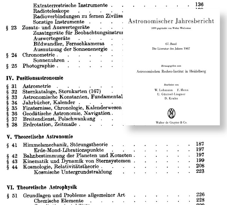
  This was how they did what I am talking about here almost 60 years ago: a page of the table of contents of the “Astronomischer Jahresbericht” for 1967, the last volume before it was turned into the English-language Astronomy and Astrophysics Abstracts, which were the main tool for literature work in astronomy until the ADS came along in the late 1990ies.

  • Thesauri and the UAT
  • Why Keywords?
  • The UAT constraint
  • Implementation

  I have recently created a pull request against pyVO to furnish the library with a new constraint to search for data and services: Search by a concept drawn from the Unified Astronomy Thesaurus UAT. This is not entirely different from the classical search by subject keywords that was what everyone did before we had the ADS, which is what I am trying to illustrate above. But it has some twists that, I would argue, still make it valuable even in the age of full-text indexes.

  To make my argument, let me first set the stage.

  Thesauri and the UAT

  (Disclaimer: I am currently a member of the UAT steering committee and therefore cannot claim neutrality. However, I would not claim neutrality otherwise, either: the UAT is not perfect, but it's already great)

  Librarians (and I am one at heart) love thesauri. Or taxonomies. Or perhaps even ontologies. What may sound like things out of a Harry Potter novel are actually ways to organise a part of the world (a “domain”) into “concepts”. If you are suitably minded, you can think of a “concept“ as a subset of the domain; “suitably minded“ here means that you consider the world as a large set of things and a domain a subset of this world. The IVOA Vocabularies specification contains some additional philosophical background on this way of thinking in sect. 5.2.4.

  On this other hand, if you are not suitably minded, a “concept” is not much different from a topic.

  There are differences in how each of thesaurus, taxonomy, and ontology does that organising (and people don't always agree on the differences). Ontologies, for instance, let you link concepts in every way, as in “a (bicycle) (is steered) (using) a (handle bar) (made of) ((steel) or (aluminum))“; every parenthesised phrase would be a node (which is a better term in ontologies than “concept”) in a suitably general ontology, and connecting these nodes creates a fine-graned representation of knowledge about the world.

  That is potentially extremely powerful, but also almost too hard for humans. Check out WordNet for how far one can take ontologies if very many very smart people spend very many years.

  Thesauri, on the other hand, are not as powerful, but they are simpler and within reach for mere humans: there, concepts are simply organised into something like a tree, perhaps (and that is what many people would call a taxonomy) using is-a relationships: A human is a primate is a mammal is a vertebrate is an animal. The UAT actually is using somewhat vaguer notions called “narrower” and “wider”. This lets you state useful if somewhat loose relationships like “asteroid-rotation is narrower than asteroid-dynamics”. For experts: The UAT is using a formalism called SKOS; but don't worry if you can't seem to care.

  The UAT is standing on the shoulders of giants: Before it, there has been the IAU thesaurus in 1993, and an astronomy thesaurus was also produced under the auspices of the IVOA. And then there were (and to some extent still are) the numerous keyword schemes designed by journal publishers that would also count as some sort of taxonomy or astronomy.

  “Numerous” is not good when people have to assign keywords to their journal articles: If A&A use something drastically or only subtly different from ApJ, and MNRAS still something else, people submitting to multiple journals will quite likely lose their patience and diligence with the keywords. For reasons I will discuss in a second, that is a shame.

  Therefore, at least the big American journals have now all switched to using UAT keywords, and I sincerely hope that their international counterparts will follow their example where that has not already happened.

  Why Keywords?

  Of course, you can argue that when you can do full-text searches, why would you even bother with controlled keyword lists? Against that, I would first argue that it is extremely useful to have a clear idea of what a thing is called: For example, is it delta Cephei stars, Cepheids, δ Cep stars or still something else? Full text search would need to be rather smart to be able to sort out terminological turmoil of this kind for you.

  And then you would still not know if W Virginis stars (or should you say “Type II Cepheids”? You see how useful proper terminology is) are included in whatever your author called Cepheids (or whatever they called it). Defining concepts as precisely as possible thus is already great.

  The keyword system becomes even more useful when the hiearchy we see in the Cepheid example becomes visible to computers. If a computer knows that there is some relationship between W Virgins stars and classical Cepheids, it can, for instance, expand or refine your queries (“give me data for all kinds of Cepheids”) as necessary. To give you an idea of how this looks in practice, here is how SemBaReBro displays the Cepheid area in the UAT:

  

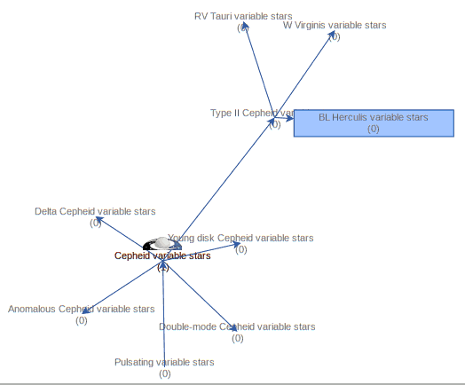
  In that image, only concepts associated with resources in the Registry have a spiffy IVOA logo; that so few VO resources claim to deal with Cepheids tells you that our data providers can probably improve their annotations quite a bit. But that is for another day; the hope is that as more people search using UAT concepts, the data providers will see a larger benefit in choosing them wisely[1].

  By the way, if you are a regular around here, you will have seen images like that before; I have talked about Sembarebro in 2021 already, and that post contains more reasons for having and maintaining vocabularies.

  Oh, and for the definitions of the concepts, you can (in general; in the UAT, there are still a few concepts without definitions) dereference the concept URI, which in the VO is always of the form <vocabulary uri>#<term identifier>, where the vocabulary URI starts with http://www.ivoa.net/rdf, after which there is the vocabulary name.

  Thus, if you point your web browser to https://www.ivoa.net/rdf/uat#cepheid-variable-stars[2], you will learn that a Cepheid is:

  A class of luminous, yellow supergiants that are pulsating variables and whose period of variation is a function of their luminosity. These stars expand and contract at extremely regular periods, in the range 1-50 days [...]

  The UAT constraint

  Remember? This was supposed to be a blog post about a new search constraint in pyVO. Well, after all the preliminaries I can finally reveal that once pyVO PR #649 is merged, you can search by UAT concepts:

  >>> from pyvo import registry
  >>> print(registry.search(registry.UAT("variable-stars")))
  <DALResultsTable length=2010>
                ivoid               ...
                                    ...
                object              ...
  --------------------------------- ...
           ivo://cds.vizier/b/corot ...
            ivo://cds.vizier/b/gcvs ...
             ivo://cds.vizier/b/vsx ...
            ivo://cds.vizier/i/280b ...
             ivo://cds.vizier/i/345 ...
             ivo://cds.vizier/i/350 ...
                                ... ...
              ivo://cds.vizier/v/97 ...
           ivo://cds.vizier/vii/293 ...
     ivo://org.gavo.dc/apass/q/cone ...
  ivo://org.gavo.dc/bgds/l/meanphot ...
       ivo://org.gavo.dc/bgds/l/ssa ...
       ivo://org.gavo.dc/bgds/q/sia ...
  

  In case you have never used pyVO's Registry API before, you may want to skim my post on that topic before continuing.

  Since the default keyword search also queries RegTAP's res_subject table (which is what this constraint is based on), this is perhaps not too exciting. At least there is a built-in protection against typos:

  >>> print(registry.search(registry.UAT("varialbe-stars")))
  Traceback (most recent call last):
    File "<stdin>", line 1, in <module>
    File "/home/msdemlei/gavo/src/pyvo/pyvo/registry/rtcons.py", line 713, in __init__
      raise dalq.DALQueryError(
  pyvo.dal.exceptions.DALQueryError: varialbe-stars does not identify an IVOA uat concept (see http://www.ivoa.net/rdf/uat).
  

  It becomes more exciting when you start exploiting the intrinsic hierarchy; the constraint constructor supports optional keyword arguments expand_up and expand_down, giving the number of levels of parent and child concepts to include. For instance, to discover resources talking about any sort of supernova, you would say:

  >>> print(registry.search(registry.UAT("supernovae", expand_down=10)))
  <DALResultsTable length=593>
                   ivoid                   ...
                                           ...
                   object                  ...
  ---------------------------------------- ...
                     ivo://cds.vizier/b/sn ...
                   ivo://cds.vizier/ii/159 ...
                   ivo://cds.vizier/ii/189 ...
                   ivo://cds.vizier/ii/205 ...
                  ivo://cds.vizier/ii/214a ...
                   ivo://cds.vizier/ii/218 ...
                                       ... ...
             ivo://cds.vizier/j/pasp/122/1 ...
         ivo://cds.vizier/j/pasp/131/a4002 ...
             ivo://cds.vizier/j/pazh/30/37 ...
            ivo://cds.vizier/j/pazh/37/837 ...
  ivo://edu.gavo.org/eurovo/aida_snconfirm ...
                  ivo://mast.stsci/candels ...
  

  There is no overwhelming magic in this, as you can see when you tell pyVO to show you the query it actually runs:

  >>> print(registry.get_RegTAP_query(registry.UAT("supernovae", expand_down=10)))
  SELECT
    [crazy stuff elided]
  WHERE
  (ivoid IN (SELECT DISTINCT ivoid FROM rr.res_subject WHERE res_subject in (
    'core-collapse-supernovae', 'hypernovae', 'supernovae',
    'type-ia-supernovae', 'type-ib-supernovae', 'type-ic-supernovae',
    'type-ii-supernovae')))
  GROUP BY [whatever]
  

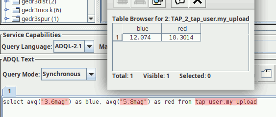
  Incidentally, some services have an ADQL extension (a “user defined function“ or UDF) that lets you do these kinds of things on the server side; that is particularly nice when you do not have the power of Python at your fingertips, as for instance interactively in TOPCAT. This UDF is:

  gavo_vocmatch(vocname STRING, term STRING, matchagainst STRING) -> INTEGER
  

  (documentation at the GAVO data centre). There are technical differences, some of which I try to explain in amoment. But if you run something like:

  SELECT ivoid FROM rr.res_subject
  WHERE 1=gavo_vocmatch('uat', 'supernovae', res_subject)
  

  on the TAP service at http://dc.g-vo.org/tap, you will get what you would get with registry.UAT("supernovae", expand_down=1). That UDF also works with other vocabularies. I particularly like the combination of product-type, obscore, and gavo_vocmatch.

  If you wonder why gavo_vocmatch does not go on expanding towards narrower concepts as far as it can go: That is because what pyVO does is semantically somewhat questionable.

  You see, SKOS' notions of what is wider and narrower are not transitive. This means that just because A is wider than B and B is wider than C it is not certain that A is wider than C. In the UAT, this sometimes leads to odd results when you follow a branch of concepts toward narrower concepts, mostly because narrower sometimes means part-of (“Meronymy”) and sometimes is-a (“Hyponymy“). Here is an example discovered by my colleague Adrian Lucy:

  interstellar-medium wider nebulae wider emission-nebulae wider planetary-nebulae wider planetary-nebulae-nuclei

  Certainly, nobody would argue that that the central stars of planetary nebulae somehow are a sort of or are part of the interstellar medium, although each individual relationship in that chain makes sense as such.

  Since SKOS relationships are not transitive, gavo_vocmatch, being a general tool, has to stop at one level of expansion. By the way, it will not do that for the other flavours of IVOA vocabularies, which have other (transitive) notions of narrower-ness. With the UAT constraint, I have fewer scruples, in particular since the expansion depth is under user control.

  Implementation

  Talking about technicalities, let me use this opportunity to invite you to contribute your own Registry constraints to pyVO. They are not particularly hard to write if you know both ADQL and Python. You will find several examples – between trivial and service-sensing complex in pyvo.registry.rtcons. The code for UAT looks like this (documentation removed for clarity[3]):

  class UAT(SubqueriedConstraint):
      _keyword = "uat"
      _subquery_table = "rr.res_subject"
      _condition = "res_subject in {query_terms}"
      _uat = None
  
      @classmethod
      def _expand(cls, term, level, direction):
          result = {term}
          new_concepts = cls._uat[term][direction]
          if level:
              for concept in new_concepts:
                  result |= cls._expand(concept, level-1, direction)
          return result
  
      def __init__(self, uat_keyword, *, expand_up=0, expand_down=0):
          if self.__class__._uat is None:
              self.__class__._uat = vocabularies.get_vocabulary("uat")["terms"]
  
          if uat_keyword not in self._uat:
              raise dalq.DALQueryError(
                  f"{uat_keyword} does not identify an IVOA uat"
                  " concept (see http://www.ivoa.net/rdf/uat).")
  
          query_terms = {uat_keyword}
          if expand_up:
              query_terms |= self._expand(uat_keyword, expand_up, "wider")
          if expand_down:
              query_terms |= self._expand(uat_keyword, expand_down, "narrower")
  
          self._fillers = {"query_terms": query_terms}
  

  Let me briefly describe what is going on here. First, we inherit from the base class SubqueriedConstraint. This is a class that takes care that your constraints are nicely encapsulated in a subquery, which generally is what you want in pyVO. Calmly adding natural joins as recommended by the RegTAP specification is a dangerous thing for pyVO because as soon as a resource matches your constraint more than once (think “columns with a given UCD”), the RegistryResult lists in pyVO will turn funny.

  To make a concrete SubqueriedConstraint, you have to fill out:

  • the table it will operate on, which is in the _subquery_table class attribute;
  • an expression suitable for a WHERE clause in the _condition attribute, which is a template for str.format. This is often computed in the constructor, but here it is just a constant expression and thus works fine as a class attribute;
  • a mapping _fillers mapping the substitutions in the _condition string template to Python values. PyVO's RegTAP machinery will worry about making SQL literals out of these, so feel free to just dump Python values in there. See the make_SQL_literal for what kinds of types it understands and expand it as necessary.

  There is an extra class attribute called _keyword. This is used by the pyvo.regtap machinery to let users say, for instance, registry.search(uat="foo.bar") instead of registry.search(registry.UAT("foo.bar")). This is a fairly popular shortcut when your constraints can be expressed as simple strings, but in the case of the UAT constraint you would be missing out on all the interesting functionality (viz., the query expansion that is only available through optional arguments to its constructor).

  This particular class has some extra logic. For one, we cache a copy of the UAT terms on first use at the class level. That is not critical for performance because caching already happens at the level of get_vocabulary; but it is convenient when we want query expansion in a class method, which in turn to me feels right because the expansion does not depend on the instance. If you don't grok the __class__ magic, don't worry. It's a nerd thing.

  More interesting is what happens in the _expand class method. This takes the term to expand, the number of levels to go, and whether to go up or down in the concept trees (which are of the computer science sort, i.e., with the root at the top) in the direction argument, which can be wider or narrower, following the names of properties in Desise, the format we get our vocabulary in. To learn more about Desise, see section 3.2 of Vocabularies in the VO 2.

  At each level, the method now collects the wider or narrower terms, and if there are still levels to include, calls itself on each new term, just with level reduced by one. I consider this a particularly natural application of recursion. Finally. everything coming back is merged into a set, which then is the return value.

  And that's really it. Come on: write your own RegTAP constraints, and also have fun with vocabularies. As you see here, it's really not that magic.

  [1]	Also, just so you don't leave with the impression I don't believe in AI tech at all, something like SciX's KAILAS might also help improving Registry subject keywords.

  [2]

  Yes, in a little sleight of hand, I've switched the URI scheme to https here. That's not really right, because the term URIs are supposed to be opaque, but some browsers currently forget the fragment identifiers when the IVOA web server redirects them to https, and so https is safer for this demonstration. This is a good example of why the web would be a better place if http had been evolved to support transparent, client-controlled encryption (rather than inventing https).

  [3]	I've always wanted to write this.

• Doing Large-Scale ADQL Queries

  2025-01-27 Markus Demleitner

  • Raising the Match Limit
  • Giving the Query More Time
  • Planning for Large Result Sets? Get in Contact!
  • Uniform-Length Partitions
  • Equal-Size Partitions

  You can do many interesting things with TAP and ADQL while just running queries returning a few thousand rows after a few seconds. Most examples you would find in tutorials are of that type, and when the right indexes exist on the queried tables, the scope of, let's say, casual ADQL goes far beyond toy examples.

  Actually, arranging things such that you only fetch the data you need for the analysis at hand – and that often is not much more than the couple of kilobytes that go into a plot or a regression or whatever – is a big reason why TAP and ADQL were invented in the first place.

  But there are times when the right indexes are not in place, or when you absolutely have to do something for almost everything in a large table. Database folks call that a sequential scan or seqscan for short. For larger tables (to give an order of magnitude: beyond 10⁷ rows in my data centre, but that obviously depends), this means you have to allow for longer run times. There are even times when you may need to fetch large portions of such a large table, which means you will probably run into hard match limits when there is just no way to retrieve your full result set in one go.

  This post is about ways to deal with such situations. But let me state already that having to go these paths (in particular the partitioning we will get to towards the end of the post) may be a sign that you want to re-think what you are doing, and below I am briefly giving pointers on that, too.

  Raising the Match Limit

  Most TAP services will not let you retrieve arbitrarily many rows in one go. Mine, for instance, at this point will snip results off at 20'000 rows by default, mainly to protect you and your network connection against being swamped by huge results you did not expect.

  You can, and frequently will have to (even for an all-sky level 6 HEALPix map, for instance, as that will retrieve 49'152 rows), raise that match limit. In TOPCAT, that is done through a little combo box above the query input (you can enter custom values if you want):

  

  If you are somewhat confident that you know what you are doing, there is nothing wrong with picking the maximum limit right away. On the other hand, if you are not prepared to do something sensible with, say, two million rows, then perhaps put in a smaller limit just to be sure.

  In pyVO, which we will be using in the rest of this post, this is the maxrec argument to run_sync and its sibling methods on TAPService.

  Giving the Query More Time

  When dealing with non-trivial queries on large tables, you will often also have to give the query some extra time. On my service, for instance, you only have a few seconds of CPU time when your client uses TAP's synchronous mode (by calling TAPService.run_sync method). If your query needs more time, you will have to go async. In the simplest case, all that takes is write run_async rather than run_sync (below, we will use a somewhat more involved API; find out more about this in our pyVO course).

  In async mode, you have two hours on my box at this point; this kind of time limit is, I think, fairly typical. If even that is not enough, you can ask for more time by changing the job's execution_duration parameter (before submitting it to the database engine; you cannot change the execution duration of a running job, sorry).

  Let us take the example of a colour-magnitude diagram for stars in Gaia DR3 with distances of about 300 pc according to Bailer-Jones et al (2021); to make things a bit more entertaining, we want to load the result in TOPCAT without first downloading it locally; instead, we will transmit the result's URI directly to TOPCAT[1], which means that your code does not have to parse and re-package the (potentially large) data.

  On the first reading, focus on the main function, though; the SAMP fun is for later:

  import time
  import pyvo
  
  QUERY = """
  SELECT
      source_id, phot_g_mean_mag, pseudocolour,
      pseudocolour_error, phot_g_mean_flux_over_error
  FROM gedr3dist.litewithdist
  WHERE
      r_med_photogeo between 290 and 310
      AND ruwe<1.4
      AND pseudocolour BETWEEN 1.0 AND 1.8
  """
  
  def send_table_url_to_topcat(conn, table_url):
      client_id = pyvo.samp.find_client_id(conn, "topcat")
      message = {
          "samp.mtype": "table.load.votable",
          "samp.params": {
              "url": table_url,
              "name": "TAP result",}
      }
      conn.notify(client_id, message)
  
  
  def main():
      svc = pyvo.dal.TAPService("http://dc.g-vo.org/tap")
      job = svc.submit_job(QUERY, maxrec=3000)
      try:
          job.execution_duration=10000  # that's 10000 seconds
          job.run()
          job.wait()
          assert job.phase=="COMPLETED"
  
          with pyvo.samp.connection(addr="127.0.0.1") as conn:
              send_table_url_to_topcat(conn, job.result_uri)
      finally:
          job.delete()
  
  if __name__=="__main__":
      main()
  

  As written, this will be fast thanks to maxrec=3000, and you wouldn't really have to bother with async just yet. The result looks nicely familiar, which means that in that distance range, the Bailer-Jones distances are pretty good:

  

  Now raise the match limit to 30000, and you will already need async. Here is what the result looks like:

  

  Ha! Numbers matter: at least we are seeing a nice giant branch now! And of course the dot colours do not represent the colours of the stars with the respective pseudocolour; the directions of blue and red are ok, but most of what you are seeing here will look rather ruddy in reality.

  You will not really need to change execution_duration here, nor will you need it even when setting maxrec=1000000 (or anything more, for that matter, as the full result set size is 330'545), as that ends up finishing within something like ten minutes. Incidentally, the result for the entire 300 pc shell, now as a saner density plot, looks like this:

  

  Ha! Numbers matter even more. There is now even a (to me surprisingly clear) horizontal branch in the plot.

  Planning for Large Result Sets? Get in Contact!

  Note that if you were after a global colour-magnitude diagram as the one I have just shown, you should probably do server-side aggregation (that is: compute the densities in a few hundred or thousand bins on the server and only retrieve those then) rather than load ever larger result sets and then have the aggregation be performed by TOPCAT. More generally, it usually pays to try and optimise ADQL queries that are slow and have huge result sets before fiddling with async and, even more, with partitioning.

  Most operators will be happy to help you do that; you will find some contact information in TOPCAT's service tab, for instance. In pyVO, you could use the get_contact method of the objects you get back from the Registry API[2]:

  >>> pyvo.registry.search(ivoid="ivo://org.gavo.dc/tap")[0].get_contact()
  'GAVO Data Centre Team (+49 6221 54 1837) <gavo@ari.uni-heidelberg.de>'
  

  That said: sometimes neither optimisation nor server-side aggregation will do it: You just have to pull more rows than the service's match limit. You see, most servers will not let you pull billions of rows in one go. Mine, for instance, will cap the maxrec at 16'000'000. What you need to do if you need to pull more than that is chunking up your query such that you can process the whole sky (or whatever else huge thing makes the table large) in manageable chunks. That is called partitioning.

  Uniform-Length Partitions

  To partition a table, you first need something to partition on. In database lingo, a good thing to partition on is called a primary key, typically a reasonably short string or, even better, an integer that maps injectively to the rows (i.e., not two rows have the same key). Let's keep Gaia as an example: the primary key designed for it is the source_id.

  In the simplest case, you can “uniformly” partition between 0 and the largest source_id, which you will find by querying for the maximum:

  SELECT max(source_id) FROM gaia.dr3lite
  

  This should be fast. If it is not, then there is likely no sufficiently capable index on the column you picked, and hence your choice of the primary key probably is not a good one. This would be another reason to turn to the service's contact address as above.

  In the present case, the query is fast and yields 6917528997577384320. With that number, you can write a program like this to split up your problem into N_PART sub-problems:

  import pyvo
  
  MAX_ID, N_PART = 6917528997577384320+1, 100
  partition_limits = [(MAX_ID//N_PART)*i
    for i in range(N_PART+1)]
  
  svc = pyvo.dal.TAPService("http://dc.g-vo.org/tap")
  main_query = "SELECT count(*) FROM ({part}) AS q"
  
  for lower, upper in zip(partition_limits[:-1], partition_limits[1:]):
    result = svc.run_sync(main_query.format(part=
      "SELECT * FROM gaia.dr3lite"
      "  WHERE source_id BETWEEN {} and {} ".format(lower, upper-1)))
    print(result)
  

  Exercise: Can you see why the +1 is necessary in the MAX_ID assignment?

  This range trick will obviously not work when the primary key is a string; I would probably partition by first letter(s) in that case.

  Equal-Size Partitions

  However, this is not the end of the story. Gaia's (well thought-out) enumeration scheme reflects to a large degree sky positions. So do, by the way, the IAU conventions for object designations. Since most astronomical objects are distributed highly unevenly on the sky, creating partitions with of equal size in identifier space will yield chunks of dramatically different (a factor of 100 is not uncommon) sizes in all-sky surveys.

  In the rather common event that you have a use case in which you need a guaranteed maximum result size per partition, you will therefore have to use two passes, first figuring out the distribution of objects and then computing the desired partition from that.

  Here is an example for how one might go about this:

  from astropy import table
  import pyvo
  
  MAX_ID, ROW_TARGET = 6917528997577384320+1, 10000000
  
  ENDPOINT = "http://dc.g-vo.org/tap"
  
  # the 10000 is just the number of bins to use; make it too small, and
  # your inital bins may already overflow ROW_TARGET
  ID_DIVISOR = MAX_ID/10000
  
  DISTRIBUTION_QUERY = f"""
  select round(source_id/{ID_DIVISOR}) as bin, count(*) as ct
  from gaia.dr3lite
  group by bin
  """
  
  
  def get_bin_sizes():
    """returns a ordered sequence of (bin_center, num_objects) rows.
    """
    # since the partitioning query already is expensive, cache it,
    # and use the cache if it's there.
    try:
      with open("partitions.vot", "rb") as f:
        tbl = table.Table.read(f)
    except IOError:
      # Fetch from source; takes about 1 hour
      print("Fetching partitions from source; this will take a while"
        " (provide partitions.vot to avoid re-querying)")
      svc = pyvo.dal.TAPService(ENDPOINT)
      res = svc.run_async(DISTRIBUTION_QUERY, maxrec=1000000)
      tbl = res.table
      with open("partitions.vot", "wb") as f:
        tbl.write(output=f, format="votable")
  
    res = [(row["bin"], row["ct"]) for row in tbl]
    res.sort()
    return res
  
  
  def get_partition_limits(bin_sizes):
    """returns a list of limits of source_id ranges exhausting the whole
    catalogue.
  
    bin_sizes is what get_bin_sizes returns (and it must be sorted by
    bin center).
    """
    limits, cur_count = [0], 0
    for bin_center, bin_count in bin_sizes:
      if cur_count+bin_count>MAX_ROWS:
        limits.append(int(bin_center*ID_DIVISOR-ID_DIVISOR/2))
        cur_count = 0
      cur_count += bin_count
    limits.append(MAX_ID)
    return limits
  
  
  def get_data_for(svc, query, low, high):
    """returns a TAP result for the (simple) query in the partition
    between low and high.
  
    query needs to query the ``sample`` table.
    """
    job = svc.submit_job("WITH sample AS "
      "(SELECT * FROM gaia.dr3lite"
      "  WHERE source_id BETWEEN {} and {}) ".format(lower, upper-1)
      +query, maxrec=ROW_TARGET)
    try:
      job.run()
      job.wait()
      return job.fetch_result()
    finally:
      job.delete()
  
  
  def main():
    svc = pyvo.dal.TAPService(ENDPOINT)
    limits = get_partition_limits(get_bin_sizes())
    for ct, (low, high) in enumerate(zip(limits[:-1], limits[1:])):
      print("{}/{}".format(ct, len(limits)))
      res = get_data_for(svc, <a query over a table sample>, low, high-1)
      # do your thing here
  

  But let me stress again: If you think you need partitioning, you are probably doing it wrong. One last time: If in any sort of doubt, try the services' contact addresses.

  [1]

  Of course, if you are doing long-running queries, you probably will postpone the deletion of the service until you are sure you have the result wherever you want it. Me, I'd probably print the result URL (for when something goes wrong on SAMP or in TOPCAT) and a curl command line to delete the job when done. Oh, and perhaps a reminder that one ought to execute the curl command line once the data is saved.

  [2]

  Exposing the contact information in the service objects themselves would be a nice little project if you are looking for contributions you could make to pyVO; you would probably do a natural join between the rr.interface and the rr.res_role tables and thus go from the access URL (you generally don't have the ivoid in pyVO service objects) to the contact role.

• A Proposal for Persistent TAP Uploads

  2024-10-11 Markus Demleitner

  • Creating and Deleting Uploads
  • Authenticated Use
  • Open Questions
  • Implemented in DaCHS

  From its beginning, the IVOA's Table Access Protocol TAP has let users upload their own tables into the services' databases, which is an important element of TAP's power (cf. our upload crossmatch use case for a minimal example). But these uploads only exist for the duration of the request. Having more persistent user-uploaded tables, however, has quite a few interesting applications.

  Inspired by Pat Dowler's 2018 Interop talk on youcat I have therefore written a simple implementation for persistent tables in GAVO's server package DaCHS. This post discusses what is implemented, what is clearly still missing, and how you can play with it.

  If all you care about is using this from Python, you can jump directly to a Jupyter notebook showing off the features; it by and large explains the same things as this blogpost, but using Python instead of curl and TOPCAT. Since pyVO does not know about the proposed extensions, the code necessarily is still a bit clunky in places, but if something like this will become more standard, working with persistent uploads will look a lot less like black art.

  Before I dive in: This is certainly not what will eventually become a standard in every detail. Do not do large implementations against what is discussed here unless you are prepared to throw away significant parts of what you write.

  Creating and Deleting Uploads

  Where Pat's 2018 proposal re-used the VOSI tables endpoint that every TAP service has, I have provisionally created a sibling resource user_tables – and I found that usual VOSI tables and the persistent uploads share virtually no server-side code, so for now this seems a smart thing to do. Let's see what client implementors think about it.

  What this means is that for a service with a base URL of http://dc.g-vo.org/tap[1], you would talk to (children of) http://dc.g-vo.org/tap/user_tables to operate the persistent tables.

  As with Pat's proposal, to create a persistent table, you do an http PUT to a suitably named child of user_tables:

  $ curl -o tmp.vot https://docs.g-vo.org/upload_for_regressiontest.vot
  $ curl -H "content-type: application/x-votable+xml" -T tmp.vot \
    http://dc.g-vo.org/tap/user_tables/my_upload
  Query this table as tap_user.my_upload
  

  The actual upload at this point returns a reasonably informative plain-text string, which feels a bit ad-hoc. Better ideas are welcome, in particular after careful research of the rules for 30x responses to PUT requests.

  Trying to create tables with names that will not work as ADQL regular table identifiers will fail with a DALI-style error. Try something like:

  $ curl -H "content-type: application/x-votable+xml" -T tmp.vot
    http://dc.g-vo.org/tap/user_tables/join
  ... <INFO name="QUERY_STATUS" value="ERROR">'join' cannot be used as an
    upload table name (which must be regular ADQL identifiers, in
    particular not ADQL reserved words).</INFO> ...
  

  After a successful upload, you can query the VOTable's content as tap_user.my_upload:

  

  TOPCAT (which is what painted these pixels) does not find the table metadata for tap_user tables (yet), as I do not include them in the “public“ VOSI tables. This is why you see the reddish syntax complaints here.

  I happen to believe there are many good reasons for why the volatile and quickly-changing user table metadata should not be mixed up with the public VOSI tables, which can be several 10s of megabytes (in the case of VizieR). You do not want to have to re-read that (or discard caches) just because of a table upload.

  If you have the table URL of a persistent upload, however, you inspect its metadata by GET-ting the table URL:

  $ curl http://dc.g-vo.org/tap/user_tables/my_upload | xmlstarlet fo
  <vtm:table [...]>
    <name>tap_user.my_upload</name>
    <column>
      <name>"_r"</name>
      <description>Distance from center (RAJ2000=274.465528, DEJ2000=-15.903352)</description>
      <unit>arcmin</unit>
      <ucd>pos.angDistance</ucd>
      <dataType xsi:type="vs:VOTableType">float</dataType>
      <flag>nullable</flag>
    </column>
    ...
  

  – this is a response as from VOSI tables for a single table. Once you are authenticated (see below), you can also retrieve a full list of tables from user_tables itself as a VOSI tableset. Enabling that for anonymous uploads did not seem wise to me.

  When done, you can remove the persistent table, which again follows Pat's proposal:

  $ curl -X DELETE http://dc.g-vo.org/tap/user_tables/my_upload
  Dropped user table my_upload
  

  And again, the text/plain response seems somewhat ad hoc, but in this case it is somewhat harder to imagine something less awkward than in the upload case.

  If you do not delete yourself, the server will garbage-collect the upload at some point. On my server, that's after seven days. DaCHS operators can configure that grace period on their services with the [ivoa]userTableDays setting.

  Authenticated Use

  Of course, as long as you do not authenticate, anyone can drop or overwrite your uploads. That may be acceptable in some situations, in particular given that anonymous users cannot browse their uploaded tables. But obviously, all this is intended to be used by authenticated users. DaCHS at this point can only do HTTP basic authentication with locally created accounts. If you want one in Heidelberg, let me know (and otherwise push for some sort of federated VO-wide authentication, but please do not push me).

  To just play around, you can use uptest as both username and password on my service. For instance:

    $ curl -H "content-type: application/x-votable+xml" -T tmp.vot \
    --user uptest:uptest \
    http://dc.g-vo.org/tap/user_tables/privtab
  Query this table as tap_user.privtab
  

  In recent TOPCATs, you would enter the credentials once you hit the Log In/Out button in the TAP client window. Then you can query your own private copy of the uploaded table:

  

  There is a second way to create persistent tables (that would also work for anonymous): run a query and prepend it with CREATE TABLE. For instance:

  

  The “error message” about the empty table here is to be expected; since this is a TAP query, it stands to reason that some sort of table should come back for a successful request. Sending the entire newly created table back without solicitation seems a waste of resources, and so for now I am returning a “stub” VOTable without rows.

  As an authenticated user, you can also retrieve a full tableset for what user-uploaded tables you have:

  $ curl --user uptest:uptest http://dc.g-vo.org/tap/user_tables | xmlstarlet fo
  <vtm:tableset ...>
    <schema>
      <name>tap_user</name>
      <description>A schema containing users' uploads. ...  </description>
      <table>
        <name>tap_user.privtab</name>
        <column>
          <name>"_r"</name>
          <description>Distance from center (RAJ2000=274.465528, DEJ2000=-15.903352)</description>
          <unit>arcmin</unit>
          <ucd>pos.angDistance</ucd>
          <dataType xsi:type="vs:VOTableType">float</dataType>
          <flag>nullable</flag>
        </column>
        ...
      </table>
      <table>
        <name>tap_user.my_upload</name>
        <column>
          <name>"_r"</name>
          <description>Distance from center (RAJ2000=274.465528, DEJ2000=-15.903352)</description>
          <unit>arcmin</unit>
          <ucd>pos.angDistance</ucd>
          <dataType xsi:type="vs:VOTableType">float</dataType>
          <flag>nullable</flag>
        </column>
        ...
      </table>
    </schema>
  </vtm:tableset>
  

  Open Questions

  Apart from the obvious question whether any of this will gain community traction, there are a few obvious open points:

  1. Indexing. For tables of non-trivial sizes, one would like to give users an interface to say something like “create an index over ra and dec interpreted as spherical coordinates and cluster the table according to it”. Because this kind of thing can change runtimes by many orders of magnitude, enabling it is not just some optional embellishment.

     On the other hand, what I just wrote already suggests that even expressing the users' requests in a sufficiently flexible cross-platform way is going to be hard. Also, indexing can be a fairly slow operation, which means it will probably need some sort of UWS interface.

  2. Other people's tables. It is conceivable that people might want to share their persistent tables with other users. If we want to enable that, one would need some interface on which to define who should be able to read (write?) what table, some other interface on which users can find what tables have been shared with them, and finally some way to let query writers reference these tables (tap_user.<username>.<tablename> seems tricky since with federated auth, user names may be just about anything).

     Given all this, for now I doubt that this is a use case sufficiently important to make all the tough nuts delay a first version of user uploads.

  3. Deferring destruction. Right now, you can delete your table early, but you cannot tell my server that you would like to keep it for longer. I suppose POST-ing to a destruction child of the table resource in UWS style would be straightforward enough. But I'd rather wait whether the other lacunae require a completely different pattern before I will touch this; for now, I don't believe many persistent tables will remain in use beyond a few hours after their creation.

  4. Scaling. Right now, I am not streaming the upload, and several other implementation details limit the size of realistic user tables. Making things more robust (and perhaps scalable) hence will certainly be an issue. Until then I hope that the sort of table that worked for in-request uploads will be fine for persistent uploads, too.

  Implemented in DaCHS

  If you run a DaCHS-based data centre, you can let your users play with the stuff I have shown here already. Just upgrade to the 2.10.2 beta (you will need to enable the beta repo for that to happen) and then type the magic words:

  dachs imp //tap_user
  

  It is my intention that users cannot create tables in your DaCHS database server unless you say these words. And once you say dachs drop --system //tap_user, you are safe from their huge tables again. I would consider any other behaviour a bug – of which there are probably still quite a few. Which is why I am particularly grateful to all DaCHS operators that try persistent uploads now.

  [1]	As already said in the notebook, if http bothers you, you can write https, too; but then it's much harder to watch what's going on using ngrep or friends.

• A Data Publisher's Diary: Wide Images in DASCH

  2024-05-03 Markus Demleitner

  

  This is the new resonse when you query the DASCH SIAP service for Aladin's default view on the horsehead nebula. As you can see, at least the returned images no longer are distributed over half of the sky (note the size of the view).

  The first reaction I got when the new DASCH in the VO service hit Aladin was: “your SIAP service is broken, it just dumps all images it has at me rather than honouring my positional constraint.”

  I have to admit I was intially confused as well when an in-view search from Aladin came back with images with centres on almost half the sky as shown in my DASCH-in-Aladin illustration. But no, the computer did the right thing. The matching images in fact did have pixels in the field of view. They were just really wide field exposures, made to “patrol” large parts of the sky or to count meteors.

  DASCH's own web interface keeps these plates out of the casual users' views, too. I am following this example now by having two tables, dasch.narrow_plates (the “narrow” here follows DASCH's nomenclature; of course, most plates in there would still count as wide-field in most other contexts) and dasch.wide_plates. And because the wide plates are probably not very helpful to modern mainstream astronomers, only the narrow plates are searched by the SIAP2 service, and only they are included with obscore.

  In addition to giving you a little glimpse into the decisions one has to make when running a data centre, I wrote this post because making a provisional (in the end, I will follow DASCH's classification, of course) split betwenn “wide” and “narrow” plates involved a bit of simple ADQL that may still be not totally obvious and hence may merit a few words.

  My first realisation was that the problem is less one of pixel scale (it might also be) but of the large coverage. How do we figure out the coverage of the various instruments? Well, to be robust against errors in the astrometric calibration (these happen), let us average; and average over the area of the polygon we have in s_region, for which there is a convenient ADQL function. That is:

  SELECT instrument_name, avg(area(s_region)) as meanarea
  FROM dasch.plates
  GROUP BY instrument_name
  

  It is the power of ADQL aggregate function that for this characterisation of the data, you only need to download a few kilobytes, the equivalent of the following histogram and table:

  

  Instrument Name	mean size [sqdeg]
  Eastman Aero-Ektar K-24 Lens on a K-1...
  Cerro Tololo 4 meter
  Logbook Only. Pages without plates.
  Roe 6-inch
  Palomar Sky Survey (POSS)
  1.5 inch Ross (short focus)	4284.199799877725
  Patrol cameras	4220.802442888225
  1.5-inch Ross-Xpress	4198.678060743206
  2.8-inch Kodak Aero-Ektar	3520.3257323233624
  KE Camera with Installed Rough Focus	3387.5206396388453
  Eastman Aero-Ektar K-24 Lens on a K-1...	3370.5283986677637
  Eastman Aero-Ektar K-24 Lens on a K-1...	3365.539790633015
  3 inch Perkin-Zeiss Lens	1966.1600884072298
  3 inch Ross-Tessar Lens	1529.7113188540836
  2.6-inch Zeiss-Tessar	1516.7996790591587
  Air Force Camera	1420.6928219265849
  K-19 Air Force Camera	1414.074101143854
  1.5 in Cooke "Long Focus"	1220.3028263587332
  1 in Cook Lens #832 Series renamed fr...	1215.1434235932702
  1-inch	1209.8102811770807
  1.5-inch Cooke Lenses	1209.7721123964636
  2.5 inch Cooke Lens	1160.1641223648048
  2.5-inch Ross Portrait Lens	1137.0908812243645
  Damons South Yellow	1106.5016573891376
  Damons South Red	1103.327982978934
  Damons North Red	1101.8455616455205
  Damons North Blue	1093.8380971825375
  Damons North Yellow	1092.9407550755682
  New Cooke Lens	1087.918570304363
  Damons South Blue	1081.7800084709982
  2.5 inch Voigtlander (Little Bache or...	548.7147592220762
  NULL	534.9269386355818
  3-inch Ross Fecker	529.9219051692568
  3-inch Ross	506.6278856912204
  3-inch Elmer Ross	503.7932693652602
  4-inch Ross Lundin	310.7279860552893
  4-inch Cooke (1-327)	132.690621660727
  4-inch Cooke Lens	129.39637516917298
  8-inch Bache Doublet	113.96821604869973
  10-inch Metcalf Triplet	99.24964308212328
  4-inch Voightlander Lens	98.07368690379751
  8-inch Draper Doublet	94.57937153909593
  8-inch Ross Lundin	94.5685388440282
  8-inch Brashear Lens	37.40061588712761
  16-inch Metcalf Doublet (Refigured af...	33.61565584978583
  24-33 in Jewett Schmidt	32.95324914757339
  Asiago Observatory 92/67 cm Schmidt	32.71623733985344
  12-inch Metcalf Doublet	31.35112644688316
  24-inch Bruce Doublet	22.10390937657793
  7.5-inch Cooke/Clark Refractor at Mar...	14.625992810622787
  Positives	12.600189007151709
  YSO Double Astrograph	10.770798601877804
  32-36 inch BakerSchmidt 10 1/2 inch r...	10.675406541122827
  13-inch Boyden Refractor	6.409447066606171
  11-inch Draper Refractor	5.134521254785461
  24-inch Clark Reflector	3.191361603405415
  Lowel 40 inch reflector	1.213284257086087
  200 inch Hale Telescope	0.18792105301170514

  For the instruments with an empty mean size, no astrometric calibrations have been created yet. To get a feeling for what these numbers mean, recall that the celestial sphere has an area of 4 π rad², that is, 4⋅180²/π or 42'000 square degrees. So, some instruments here indeed covered 20% of the night sky in one go.

  I was undecided between cutting at 150 (there is a fairly pronounced gap there) or at 50 (the gap there is even more pronounced) square degrees and provisionally went for 150 (note that this might still change in the coming days), mainly because of the distribution of the plates.

  You see, the histogram above is about instruments. To assess the consequences of choosing one cut or the other, I would like to know how many images a given cut will remove from our SIAP and ObsTAP services. Well, aggregate functions to the rescue again:

  SELECT ROUND(AREA(s_region)/100)*100 AS platebin, count(*) AS ct
  FROM dasch.plates
  GROUP BY platebin
  

  To plot such a pre-computed histogram in TOPCAT, tell the histogram plot window to use ct as the weight, and you will see something like this:

  

  It was this histogram that made me pick 150 deg² as the cutoff point for what should be discoverable in all-VO queries: I simply wanted to retain the plates in the second bar from left.

• HEALPix Maps: In General and in Gaia

  2022-12-22 Markus Demleitner

  

  A map of average Gaia colours in HEALPixes 2/83 and 2/86 (Orion south-east). This post tells you how to (relatively) quickly produce such maps.

  • Making HEALPix maps with Gaia source_ids
  • HEALPix to Screen Pixel
  • Positional Constraints using source_ids
  • Aggregating over a Non-HEALPix

  This year's puzzler for the AG Tagung turned out to be a valuable source of interesting ADQL queries. I have already written about finding dusty spots on the sky, and in the puzzler solution, I had promised some words on creating dust maps, or, more generally, HEALPix maps of any sort.

  Making HEALPix maps with Gaia source_ids

  The basic technique is explained in Mark Taylor's classical ADASS poster from 2016. On GAVO's TAP service (access URL http://dc.g-vo.org/tap), you will also find an example for that (in TOPCAT's TAP window, check the Service-provided section unter the Examples button for it). However, once you have Gaia source_ids, there is something a lot faster and arguably not much less convenient. Let me quote the footnote on source_id from my DR3 lite table:

  For the contents of Gaia DR3, the source ID consists of a 64-bit integer, least significant bit = 1 and most significant bit = 64, comprising:

  • a HEALPix index number (sky pixel) in bits 36 - 63; by definition the smallest HEALPix index number is zero.
  • […]

  This means that the HEALpix index level 12 of a given source is contained in the most significant bits. HEALpix index of 12 and lower levels can thus be retrieved as follows:

  • [...]
  • HEALpix [at] level n = (source_id)/(2³⁵⋅4^12 − n).

  That is: Once you have a Gaia source_id, you an compute HEALpix indexes on levels 12 or less by a simple integer division! I give you that the more-than-35-bit numbers you have to divide by do look a bit scary – but you can always come back here for cutting and pasting:

  HEALPix level	Integer-divide source id by
  12	34359738368
  11	137438953472
  10	549755813888
  9	2199023255552
  8	8796093022208
  7	35184372088832
  6	140737488355328
  5	562949953421312
  4	2251799813685248
  3	9007199254740992
  2	36028797018963968

  If you know – and that is very valuable knowledge far beyond this particular application – that you can simply jump between HEALPix indexes of different levels by multiplying with or integer-dividing by four, the general formula in the footnote actually becomes rather memorisable. Let me illustrate that with an example in Python. HEALPix number 3145 on level 6 is:

  >>> 3145//4  # ...within this HEALPix on level 5...
  786
  >>> 3145*4, (3145+1)*4  # ..and covers these on level 7...
  (12580, 12584)
  

  Simple but ingenious.

  You can immediately exploit this to make HEALPix maps like the one in the puzzler. This piece of ADQL does the job within a few seconds on the GAVO DC TAP service[1]:

  SELECT source_id/8796093022208 AS pix,
    AVG(phot_bp_mean_mag-phot_rp_mean_mag) AS avgcol
  FROM gaia.edr3lite
  WHERE distance(ra, dec, 246.7, -24.5)<2
  GROUP by pix
  

  Using the table above, you see that the horrendous 8796093022208 is the code for HEALPix level 8. When you remember (and you should) that HEALPix level 6 corresponds to a linear dimension of about 1 degree and each level is a factor of two in linear dimension, you see that the map ought to have a resolution of about 1/8th of a degree.

  HEALPix to Screen Pixel

  How do you plot this? Well, in TOPCAT, do Graphics → Sky Plot, and then in the plot window Layers → Add HEALPix control (there are icons for both of these, too). You then have to manually configure the plot for the table you just retrieved: Set the Level to 8, the index to pix and the Value to avgcol – we're working on making the annotation a bit richer so that TOPCAT has a chance to figure this out by itself.

  With a bit of extra configuration, you get the following map of average colours (really: dust concentration):

  

  This is not totally ideal, as at the border of the cone, certain Healpixes are only partially covered, which makes statistics unnecessarily harder.

  Positional Constraints using source_ids

  Due to Gaia's brilliant numbering scheme, we can do analysis by HEALpix, too, circumventing (among other things) this problem. Say you are interested in the vicinity of the M42 and would like to investigate a patch of about 8 degrees. By our rule of thumb, 8 degrees is three levels up from the one-degree level 6. To find the corresponding HEALpix index, on DaCHS servers with their gavo_simbadpoint UDF you could say:

  SELECT TOP 1 ivo_healpix_index(3, gavo_simbadpoint('M42'))
  FROM tap_schema.tables
  

  Hu, you ask, what's tap_schema.tables to do with this? Well, nothing, really. It's just that ADQL's syntax requires selecting from a table, even if what we select is completely independent of any table, as for instance the index of M42's 3-HEALpix. The hack above picks in a table guaranteed to exist on all TAP services, and the TOP 1 makes sure we only compute the value once. In case you ever feel the need to abuse a TAP service as a calculator: Keep this trick in mind.

  The result, 334, you could also have found more graphically, as follows:

  1. Start Aladin
  2. Check Overlay → HEALPix grid
  3. Enter M42 in Command
  4. Zoom out until you see HEALPix indexes of level 3 in the grid.

  An advantage you have with this method: You see that M42 happens to lie on a border of HEALPixes; perhaps you should include all of 334, 335, 356, and 357 if you were really interested in the Orion Nebula's vicinity.

  We, on the other hand, are just interested in instructive examples, and hence let's just repeat our colour mapping with all Gaia objects from HEALPix 3/334. How do you select these? Well, by source_id's construction, you know their source_ids will be between 334⋅9007199254740992 and (334 + 1)⋅9007199254740992 − 1:

  SELECT source_id/8796093022208 AS pix,
    AVG(phot_bp_mean_mag-phot_rp_mean_mag) AS avgcol
  FROM gaia.edr3lite
  WHERE source_id BETWEEN 334*9007199254740992 AND 335*9007199254740992-1
  GROUP by pix
  

  This is computationally cheap (though Postgres, not being a column store still has to do quite a bit of I/O; note how much faster this query is when you run it again and all the tuples are already in memory). Even going to HEALPix level 2 would in general still be within our sync time limit. The opening figure was produced with the constraint:

  source_id BETWEEN 83*36028797018963968 AND 84*36028797018963968-1
  OR source_id BETWEEN 86*36028797018963968 AND 87*36028797018963968-1
  

  – and with a sync query.

  Aggregating over a Non-HEALPix

  One last point: The constraints we have just been using are, in effect, positional constraints. You can also use them as quick and in some sense rather unbiased sampling tools.

  For instance, if you would like so see how the reddening in one of the “dense“ spots in the opening picture behaves with distance, you could first pick a point – α = 98, δ = 4, say –, then convert that to a level 7 healpix as above (that's/88974) and then write:

  SELECT ROUND(r_med_photogeo/200)*200 AS distbin, COUNT(*) as n,
      AVG(phot_bp_mean_mag-phot_rp_mean_mag) AS avgcol
  FROM gaia.dr3lite
  JOIN gedr3dist.main USING (source_id)
  WHERE source_id BETWEEN 88974*35184372088832 and 88975*35184372088832-1
  GROUP BY distbin
  

  This is creating 200 pc bins in distance based on the estimates in the gedr3dist.main table (note that this adds subtle correlations, because these estimates already contain Gaia colour information). Since quite a few of these bins will be very sparsely populated, I'm also fetching the number of objects contributing. And then I plot the whole thing, using the conventional √(n) ⁄ n as a rough estimate for the relative error:

  

  This plot immediatly shows that colour systematics are not exclusively due to dust, as in that case things would only get redder all the time. The blueward trend up to 700 pc is reasonably well explained by the brighter, bluer upper main sequence becoming more dominant in the population sampled as red dwarfs become too faint for Gaia.

  The strong reddening setting in after that is rather certainly due to the Orion complex, though I would perhaps not have expected it to reach out to 2 kpc (the conventional distance to M42 is about 0.5 kpc); without having properly thought about it, I'll chalk it off as “the Orion arm“. And after that, it's again what I'd call Malmquist-blueing until the whole things dissolves into noise.

  In conclusion: Did you know you can group by both healpix and distbin at the same time? I am sure there are interesting structures to be found in what you will get from such a query…

  [1]

  You may be tempted to write source_id/(POWER(2, 35)*POWER(4, 3) here for clarity. Resist that temptation. POWER returns floating point numbers. If you have one float in a division, not even a ROUND will get you back into the integer division realm, and the whole trick implodes. No, you will need the integer literals for now.

Page 1 / 3 »