Posts with the Tag Time series:

• DaCHS 2.2 is out

  2020-10-13 Markus Demleitner

  

  DaCHS 2.2 adds support for what simple semantics we currently do in the VO. Which is a welcome excuse to abuse one of the funny symbols semanticians love so much.

  Today, I've released DaCHS 2.2, the second stable version of DaCHS running on Python 3. Indeed, we have ironed out a few sore spots that have put that “stable” into question, especially if you didn't run things on Debian Buster. Mind you, playing it safe and just going for Debian is still recommended: Compared to the Python 2 world, where things largely didn't break for a decade, the Python 3 universe is still shaking out, and so the versions of dependencies do matter. It's actually fairly gruesome how badly pyparsing 2.4 will break DaCHS. But that's for another day.

  Despite this piece of fearmongering, it'd be great if you could upgrade your installations if you are running DaCHS, and it's pretty safe if you're on Debian buster anyway (and if you're running Debian in the first place, you should be running buster by now).

  Here are the more notable changes in this release:

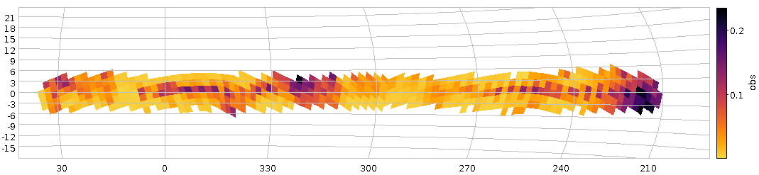
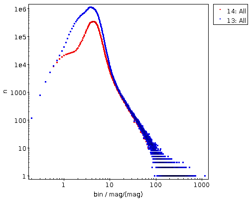
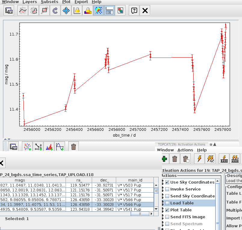
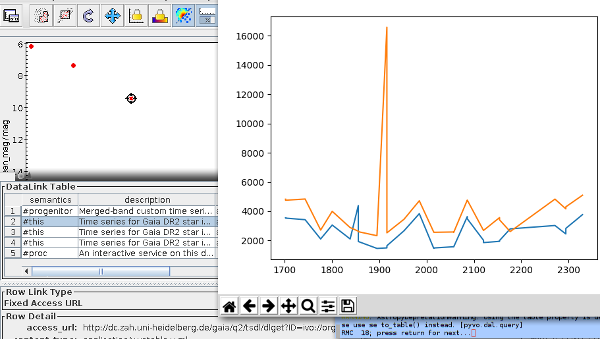
  • DaCHS can now (relatively easily) write time series in the form of what Ada Nebot's Time Series Annotation note proposes. See the tutorial chapter on building time series for how to do that in practice. Seriously: If you have time series to publish, by all means try this out. The specification can still be fixed, and so this is the perfect time to find problems with the plan.
  • The 2.2 release contains support for the MOC ADQL functions mentioned in the last post on this blog. Of course, to make them work, you will still have to acquaint your database with the new functionality.
  • DaCHS has learned to use IVOA vocabularies as per the current draft for Vocabularies in the VO 2. The most visible effect for you probably is that DaCHS now warns if your subject keywords are not taken from the Unified Astronomy Thesaurus (UAT) – which they almost certainly are not, because the actual format of these keywords is a bit funky. On the other hand, if you employ the “plain” root page template (see the root template in our templating guide if you are not sure what I am talking about here), you will get nice, human-friendly labels for the computer-friendly terms you ought to put into subjects. In case you don't bother: Given I'm currently serving as chair of the semantics working group of the IVOA, the whole topic will certainly come up again soon, and at that point I will probably also talk about another semantics-related newcomer to DaCHS, the gavo_vocmatch ADQL UDF.
  • There is a new command dachs datapack for interacting with frictionless data packages. The idea is that you can say dachs datapack create myres/q myres.pack and obtain an archive of all that is necessary to re-create myres on another DaCHS installation, where you would say dachs datapack load myres.pack. Frankly, this isn't much different from just tarring up the resource directory at this point, except that any cruft that may have accumulated in the directory is skipped and there is a bit of structured metadata. But then interoperability always starts slowly. Note, by the way, that this certainly does not teach DaCHS to do anything sensible with third-party data packages; while I've not thought hard about this, as it seems a remote use case, I am pretty sure that even the “tabular data packages” that refine the rough general metadata quite a bit simply have nowhere near enough metadata to create a useful VO resource or TAP table.
  • As part of my never-ending struggle against bitrot (in case you've always wondered what “curation” means: that, essentially), I'm running dachs val -vc ALL in my own data center once every month. This used to traverse the file system to locate all RDs defined on a box and then make sure they are still ok and their definitions match the database schema. That behaviour has now changed a bit: It will only check published RDs now. I cannot lie: the main reason for the change is because on my production machine the file system traversal has taken longer and longer as data accumulated. But then beyond that there is much less to worry when unpublished gets a little bit mouldy. To get back the old behaviour of validating all RDs that are reachable by the server, use ALL_RECURSE instead of ALL.
  • DaCHS has traditionally assumed that you are running multiple services on one site, which is why its root page is rendered over a service that exposes metadata on local resources. If that doesn't quite work for how you use DaCHS – perhaps because you want to have your own custom renderers and data functions on your root page, perhaps because you only have one browser-based service and that should be the root page right away –, you can now override what is shown when people access the root URI of your DaCHS installation by setting the [web]root config item to the path of the resource you want as root (e.g., myres/q/s/fixed when the root page should be made by the fixed renderer on the service s within the RD myres/q).
  • Scripting in DaCHS is a powerful way to execute python or SQL code when certain things happen. That seems an odd thing to want until you need it; then you need it badly. Since DaCHS 2.2, scripts executed before or after the creation of a table, before its deletion, or after its meta data has been updated, can sit on tables (where they have always belonged). Before, they could only be on makes (where they can still sit, but of course they are then only executed if the table is operated through that particular make) and RDs (from where they could be copied). That latter location is now forbidden in order to free up RD scripts for later sanitation. Use STREAM and FEED instead if you really used something like that (and I'd bet you don't).
  • Minor behavioural changes:
    1. Due to a bug, you could write things like <schema foo="bar">my_schema<schema>, i.e., have attributes on attributes written in element form. That is now flagged as an error. Since that attribute was fed to the embedding element, you might need to add it there.
    2. If you have custom flot plots in one of your templates (and you don't if you don't know what I'm talking about), you now have to set style to Points or Lines where you had usingIndex 0 or 1 before.
    3. The sidebar template no longer has links to a privacy policy (that few bothered to fill out). See extra sidebar items in the tutorial on how to get them back or add something else.

  The most important change comes last: The default logo DaCHS shows unless you override it is no longer the GAVO logo. That's, really, been inappropriate from the start. It's now the DaCHS logo, the thing that's in this posts's article image. Which isn't quite as tasteful as the GAVO one, true. But I trust we'll all get used to it.

• The Bochum Galactic Disk Survey

  2020-04-01 Markus Demleitner

  

  Fig 1: How our haphazard variability ratio varies over the sky (galactic coordinates). And yes, it's clear that this isn't dominated by physical variability.

  About a year ago, I reported on a workshop on “Large Surveys with Small Telescopes” in Bamberg; at around the same time, I've published an example for those, the Bochum Galactic Disk Survey BGDS, which used a twin 15 cm robotic telescope in some no longer forsaken place in the Andes mountains to monitor the brighter stars in the southern Milky Way. While some tables from an early phase of the survey have been on VizieR for a while, we now publish the source images (also in SIAP and Obscore), the mean photometry (via SCS and TAP) and, perhaps potentially most fun of all, the the lightcurves (via SSAP and TAP) – a whopping 35 million of the latter.

  This means that in tools like Aladin, you can now find such light curves (and images in two bands from a lot of epochs) when you are in the survey's coverage, and you can run TAP queries on GAVO's http://dc.g-vo.org/tap server against the full photometry table and the time series.

  Regular readers of this blog will not be surprised to see me use this as an excuse to show off a bit of ADQL trickery.

  If you have a look at the bgds.phot_all table in your favourite TAP client, you'll see that it has a column amp, giving the difference between the highest and lowest magnitude. The trouble is that amp for almost all objects just reflects the measurement error rather than any intrinsic variability. To get an idea what's “normal” (based on the fact that essentially all stars have essentially constant luminosity on the range and resolution scales considered here), run a query like:

  SELECT ROUND(amp/err_mag*10)/10 AS bin, COUNT(*) AS n
  FROM bgds.phot_all
  WHERE nobs>10
  GROUP BY bin
  

  As this scans the entire 75 million rows of the table, you will probably have to use async mode to run this.

  

  Figure 2: The distribution of amplitude over magnitude error for all BGDS objects with nobs>10 (blue) and the subset with a mean magnitude brighter than 15 (blue).

  When it comes back, you will have, for objects where any sort of statistics make sense at all (hence nobs>10), a histogram (of sorts) of the amplitude in units of upstream's magnitude error estimation. If you log-log-plot this, you'll see something like Figure 2. The curve at least tells you that the magnitude error estimate is not very far off – the peak at about 3 “sigma” is not unreasonable since about half of the objects have nobs of the order of a hundred and thus would likely contain outliers that far out assuming roughly Gaussian errors.

  And if you're doing a rough cutoff at amp/magerr>10, you will get perhaps not necessarily true variables, but, at least potentially interesting objects.

  Let's use this insight to see if we spot any pattern in the distribution of these interesting objects. We'll use the HEALPix technique I've discussed three years ago in this blog, but with a little twist from ADQL 2.1: The Common Table Expressions or CTEs I have already mentioned in my blog post on ADQL 2.1 and then advertised in the piece on the Henry Draper catalogue. The brief idea, again, is that you can write queries and give their results a name that you can use elsewhere in the query as if it were an actual table. It's not much different from normal subqueries, but you can re-use CTEs in multiple places in the query (hence the “common”), and they are usually more readable.

  Here, we first create a version of the photometry table that contains HEALPixes and our variability measure, use that to compute two unsophisticated per-HEALPix statistics and eventually join these two to our observable, the ratio of suspected variables to all stars observed (the multiplication with 1.0 is a cheap way to make a float out of a value, which is necessary here because a/b does integer division in ADQL if a and b are both integers):

  WITH photpoints AS (
    SELECT
      amp/err_mag AS redamp,
      amp,
      ivo_healpix_index(5, ra, dec) AS hpx
    FROM bgds.phot_all
    WHERE
      nobs>10
      AND band_name='SDSS i'
      AND mean_mag<16),
  all_objs AS (
    SELECT count(*) AS ct,
      hpx
      FROM photpoints GROUP BY hpx),
  strong_var AS (
    SELECT COUNT(*) AS ct,
      hpx
      FROM photpoints
      WHERE redamp>4 AND amp>1 GROUP BY hpx)
  SELECT
    strong_var.ct/(1.0*all_objs.ct) AS obs,
    all_objs.ct AS n,
    hpx
  FROM strong_var JOIN all_objs USING (hpx)
  WHERE all_objs.ct>20
  

  If you plot this using TOPCAT's HEALPix thingy and ask it to use Galactic coordinates, you will end up with something like Figure 1.

  There clearly is some structure, but given that the variables ratio reaches up to 0.2, this must be reflecting instrumental or pipeline effects and thus earthly rather than astrophysical causes. And that's going beyond what I wouldd like to talk about on a VO blog, although I'll take any bet that you will see significant structure in the spatial distribution of the variability ratio at about any magnitude cutoff, since there are a lot of different population mixtures in the survey's footprint.

  Before winding down, let's have a quick look at the time series. As with the short spectra from Byurakan use case, we have stored the actual time series as arrays in the database (the mjd and mags columns in bgds.ssa_time_series). Unfortunately, since they are a lot less array-like than homogeneous spectra, it's also a lot harder to do interesting things with them without downloading them (I'm grateful for ideas for ADQL functions that will let you do in-DB analysis for such things). Still, you can at least easily download them in bulk and then process them in, say, python to your heart's content. The Byurakan use case should give you a head start there.

  For a quick demo, I couldn't resist checking out objects that Simbad classifies as possible long-period variables (you see, as I write this, the public excitement over Betelgeuse's brief waning is just dying down), and so I queried Simbad for:

  SELECT ra, dec, main_id
  FROM basic
  WHERE
    otype='LP?'
    AND 1=CONTAINS(
       POINT('', ra, dec),
       POLYGON('', 127, -30, 112, -30, 272, -30, 258, -30))
  

  (as of this writing, Simbad still needs the ADQL 2.0-compliant first arguments to POINT and POLYGON), where the POLYGON is intended to give the survey's footprint. I obtained that by reading off the coordinates of the corners in my Figure 1 while it was still in TOPCAT. Oh, and I had to shrink it a bit because Simbad (well, the underlying Postgres server, and, more precisely, its pg_sphere extension) doesn't want polygons with edges longer than π. This will soon become less pedestrian: MOCs in relational databases are coming; more on this in a later post.

  

  Fig 3: V566 Pup's BGDS lightcuve in a TOPCAT configured to auto-plot the light curves associated with a row from the bgds.ssa_time_series table on the GAVO DC TAP service.

  If you now do the usual spiel with an upload crossmatch to the bgds.ssa_time_series table and check “Plot Table” in Views/Activation Action, you can quickly page through the light curves (TOPCAT will keep the plot style as you go from dataset to dataset, so it's worth configuring the lines and the error bars). Which could bring you to something like Fig. 3; and that would suggest that V* V566 Pup may be long-period (perhaps we are watching a slow maximium here), but on top of that there probably much faster ripples – unless the errors are grossly off; I am amazed that you can apparently do photometry at error levels of a dozen millimags or so from the ground these days.

• DaCHS 1.3 is out

  2019-05-28 Markus Demleitner

  

  Almost a year has passed since release 1.2 of DaCHS – I've let the normal autumn release slip last year because there weren't so many release-worthy new features in DaCHS at the traditional release time (i.e., after the College Park interop), and also because running betas when you do need a new feature is a fairly stable thing by now.

  But here it finally is: Release 1.3 (tarball for the die-hard self-builders; everyone else just switches back the release branch as necessary and then runs an update/upgrade cycle).

  Here's the commented changelog:

  • New //ssap#view mixin that should be used for future SSAP services, and that existing SSAP services should migrate to at some point. See A new view on SSAP in DaCHS on this blog for details.
  • Columns can now be hidden from TAP/ADQL (and other interfaces) by setting hidden="True".
  • There is now a setting [web]maxSyncUploadSize=500000 (meaning: about 500 kByte) as the default upload limit on sync queries. In compensation, clients uploading too much now receive a more useful error message (except it doesn't reach TOPCAT users most of the time because it does chunked uploads). To get back the behaviour of 1.2 (which is probably ok if you can live with the occasional resource hog), add maxSyncUploadSize=20000000 to your /etc/gavo.rc.
  • Adding support for https (certificate reading, certificate updating with letsencrypt, registering alternate endpoints, no WebSAMP with https). See HTTPS in DaCHS on this blog for details.
  • New source_table and preview columns in obscore. If you're using the various obscore mixins, this should be automatic. If you have defined views manually, you will have to amend these (and have a broken obscore until a dachs upgrade ran without error).
  • No longer producing arraysize="1" in VOTables for scalars (except char, for compatibility with a legacy TOPCAT workaround; see VOTable 1.3 Erratum 3 for background information).
  • Support for draft TIMESYS in VOTable (with STC 2 annotation; ask about details if you're interested. This is for draft VOTable 1.4 and probably only relevant to you if you're publishing time series).
  • You can now add targetType and targetTitle properties to URL-valued columns to help Aladin figure out what to do with URLs (see Datalinks as product URLs in the reference documentation).
  • New gavo_transform, gavo_ipix, and gavo_urlescape ufuncs for ADQL, fixed gavo_urlescape to have acceptable performance.
  • New generating CatalogResource records with auxiliary capabilities in accordance with Oct 2018 VODataService WD.
  • //soda#sdm_genDesc now matches accref rather than pubDID by default. If you use Datalink with SSA and have a custom pubDID schema (or no index on accref), add a useAccref="False" to your descriptorGenerator statement.
  • There is now a --foreground option for dachs serve start. This is mainly to play nice with systemd, and indeed, the Debian package now comes with a systemd unit file. I'm not terribly familiar with systemd, so please have an eye on DaCHS controlled by systemd and let me know if you see something that's not as it should be.
  • Fixes for various bugs (most notably: escaped quotes in ADQL, WCS in SIAP cutout products) and many minor improvements. Check out the source tree (still via subversion) and read the changelog if you want to know the whole truth.

  On systems running from the Debian package, the update should be automatic with the next system upgrade. However, you'll be saving yourself quite a bit of headache if you check the health of your installation before the upgrade; see Upgrading DaCHS in the operator's guide on how to upgrade professionally.

• Gaia DR2: A light version and light curves

  2018-05-07 Markus Demleitner

  

  Topcat is doing datalink, and our little python script has plotted a two-color time series of RMC 18 (or so I think).

  If anyone ever writes a history of the VO, the second data release of Gaia on April 25, 2018 will probably mark its coming-of-age – at least if you, like me, consider the Registry the central element of the VO. It was spectacular to view the spike of tens of Registry queries per second right around 12:00 CEST, the moment the various TAP services handing out the data made it public (with great aplomb, of course).

  In GAVO's Data Center we also carry Gaia DR2 data. Our host institute, the Zentrum für Astronomie in Heidelberg, also has a dedicated Gaia server. This gives relieves us from having to be a true mirror of the upstream data release. And since the source catalog has lots and lots of columns that most users will not be using most of the time, we figured a “light” version of the source catalog might fill an interesting ecological niche: Behold gaia.dr2light on the GAVO DC TAP service, containing essentially just the basic astrometric parameters and the diagonal of the covariance matrix.

  That has two advantages: Result sets with SELECT * are a lot less unwieldy (but: just don't do this with Gaia DR2), and, more importantly, a lighter table puts less load on the server. You see, conventional databases read entire rows when processing data, and having just 30% of the columns means we will be 3 times faster on I/O-bound tasks (assuming the same hardware, of course). Hence, and contrary to several other DR2-carrying sites, you can perform full sequential scans before timing out on our TAP service on gaia.dr2light. If, on the other hand, you need to do debugging or full-covariance-matrix error calculations: The full DR2 gaia_source table is available in many places in the VO. Just use the Registry.

  Photometry via TAP

  A piece of Gaia DR2 that's not available in this form anywhere else is the lightcurves; that's per-transit photometry in the G, BP, and RP band for about 0.5 million objects that the reduction system classified as variable. ESAC publishes these through datalink from within their gaia_source table, and what you get back is a VOTable that has the photometry in the three bands interleaved.

  I figured it might be useful if that data were available in a TAP-queriable table with lightcurves in the database. And that's how gaia.dr2epochflux came into being. In there, you have three triples of arrays: the epochs (g_transit_time, bp_obs_time, and rp_obs_time), the fluxes (g_transit_flux, bp_flux, and rp_flux), and their errors (you can probably guess their names). So, to retrieve G lightcurves where available together with a gaia_source query of your liking, you could write something like:

  SELECT g.*, g_transit_time, g_transit_flux
  FROM gaia.dr2light AS g
  LEFT OUTER JOIN gaia.dr2epochflux
  USING (source_id)
  WHERE ...whatever...
  

  – the LEFT OUTER JOIN arranges things such that the g_transit_time and g_transit_flux columns simply are NULL when there are no lightcurves; with a normal (“inner”) join, rows without lightcurves would not be returned in such a query.

  To give you an idea of what you can do with this, suppose you would like to discover new variable blue supergiants in the Gaia data (who knows – you might discover the precursor of the next nearby supernova!). You could start with establishing color cuts and train your favourite machine learning device on light curves of variable blue supergiants. Here's how to get (and, for simplicity, plot) time series of stars classified as blue supergiants by Simbad for which Gaia DR2 lightcurves are available, using pyvo and a little async trick:

  from matplotlib import pyplot as plt
  import pyvo
  
  def main():
    simbad = pyvo.dal.TAPService(
      "http://simbad.u-strasbg.fr:80/simbad/sim-tap")
    gavodc = pyvo.dal.TAPService("http://dc.g-vo.org/tap")
  
    # Get blue supergiants from Simbad
    simjob = simbad.submit_job("""
      select main_id, ra, dec
      from basic
      where otype='BlueSG*'""")
    simjob.run()
  
    # Get lightcurves from Gaia
    try:
      simjob.wait()
      time_series = gavodc.run_sync("""
        SELECT b.*, bp_obs_time, bp_flux, rp_obs_time, rp_flux
        FROM (SELECT
           main_id, source_id, g.ra, g.dec
           FROM
          gaia.dr2light as g
           JOIN TAP_UPLOAD.t1 AS tc
           ON (0.002>DISTANCE(tc.ra, tc.dec, g.ra, g.dec))
        OFFSET 0) AS b
        JOIN gaia.dr2epochflux
        USING (source_id)
        """,
        uploads={"t1": simjob.result_uri})
    finally:
      simjob.delete()
  
    # Now plot one after the other
    for row in time_series.table:
      plt.plot(row["bp_obs_time"], row["bp_flux"])
      plt.plot(row["rp_obs_time"], row["rp_flux"])
      plt.show(block=False)
      raw_input("{}; press return for next...".format(row["main_id"]))
      plt.cla()
  
  if __name__=="__main__":
    main()
  

  If you bother to read the code, you'll notice that we transfer the Simbad result directly to the GAVO data center without first downloading it. That's fairly boring in this case, where the table is small. But if you have a narrow pipe for one reason or another and some 10⁵ rows, passing around async result URLs is a useful trick.

  In this particular case the whole thing returns just four stars, so perhaps that's not a terribly useful target for your learning machine. But this piece of code should get you started to where there's more data.

  You should read the column descriptions and footnotes in the query results (or from the reference URL) – this tells you how to interpret the times and how to make magnitudes from the fluxes if you must. You probably can't hear it any more, but just in case: If you can, process fluxes rather than magnitudes from Gaia, because the errors are painful to interpret in magnitudes when the fluxes are small (try it!).

  Note how the photometry data is stored in arrays in the database, and that VOTables can just transport these. The bad news is that support for manipulating arrays in ADQL is pretty much zero at this point; this means that, when you have trained your ML device, you'll probably have to still download lots and lots of light curves rather than write some elegant ADQL to do the filtering server-side. However, I'd be highly interested to work out how some tastefully chosen user defined functions might enable offloading at least a good deal of that analysis to the database. So – if you know what you'd like to do, by all means let me know. Perhaps there's something I can do for you.

  Incidentally, I'll talk a bit more about ADQL arrays in a blog post coming up in a few weeks (I think). Don't miss it, subscribe to our feed).

  Datalink

  In the results from queries involving gaia.dr2epochflux, we also provide datalinks. These let you retrieve lightcurves that already have mags and that are more easily plotted. Perhaps more importantly, they link back to the full ESAC lightcurves that, in addition, give you a lot more debug information and are required if you want to reliably identify photometry points with the identifiers of the transits that generated them.

  Datalink support in clients still is not great, but it's growing nicely. Your ideas for workflows that should be supported are (again) most welcome – and have a good chance of being adopted. So, try things out, for instance by getting the most recent TOPCAT (as of this writing) and do the following:

  1. Open the VO/TAP dialog from the menu bar and double click the GAVO DC TAP service.

  2. Enter:

       SELECT source_id, ra, dec,
       phot_bp_mean_mag, phot_rp_mean_mag, phot_g_mean_mag,
       g_transit_time, g_transit_flux,
       rp_obs_time, rp_flux
       FROM gaia.dr2epochflux
       JOIN gaia.dr2light
       USING (source_id)
       WHERE parallax>50
     
     into “ADQL” text to retrieve lightcurves for the more nearby
     variables (in reality, you'd have to be a bit more careful with the
     distances, but you already knew that).
     

  3. plot something like phot_bp_mean_mag-phot_rp_mean_mag vs. phot_g_mean_mag (and adapt the plot to fit your viewing habits).

  4. Open the dialog for Views/Activation Actions (from the menu bar or the tool bar – same thing), check “Invoke Service”, choose “View Datalink Table”.

  5. Whenever you click on a a point in your CMD, a window will pop up in which you can choose between the time series in the various bands, and you can pull in the data from ESAC; to load a table, select “Load Table” from the actions near the foot of the datalink table and click “Invoke”.

  Yeah. It's clunky. Help us make it better with your fresh ideas for interfaces (and don't be cross with us if we have to marry them with what's technically feasible and readily generalised).

  SSAP and Obscore

  If you're fed up with bleeding-edge tech, the light curves are also available through good old SSAP and Obscore. To use that, just get Splat (or another SSA client, preferably with a bit of time series support). Look for a Gaia DR2 time series service (you may have to update the service list before you find it), enter (in keeping with our LBV theme) S Dor as position and hit “Lookup” followed by “Send Query”. Just click on any result to just view the time series – and then apply Splat's rich tool set to it.

  Update (8.5.2018): Clusters

  Here's another quick application – how about looking for variable stars in clusters? This piece of ADQL should get you started:

  SELECT TOP 100
    source_id, ra, dec, parallax, g.pmra, g.pmdec,
    m.name, m.pmra AS c_pmra, m.pmde AS c_pmde,
    m.e_pm AS c_e_pm,
    1/dist AS cluster_parallax
  FROM
    gaia.dr2epochflux
    JOIN gaia.dr2light AS g USING (source_id)
    JOIN mwsc.main AS m
    ON (1=CONTAINS(
      POINT(g.ra, g.dec),
      CIRCLE(m.raj2000, m.dej2000, rcluster)))
  WHERE IN_UNIT(pmdec, 'deg/yr') BETWEEN m.pmde-m.e_pm*3 AND m.pmde+m.e_pm*3
  

  – yes, you'll want to constrain pmra, too, and the distance, and properly deal with error and all. But you get simple lightcurves for free. Just add them in the SELECT clause!

• Time Series

  2017-05-03 Markus Demleitner

  The IOVA's committee on science priorities (CSP) has declared the “time domain” as one of its focus topics quite a while ago, an action boiling down to a call to the IVOA member projects to think about support for time series and their analysis in services, standards, and clients.

  While for several years, response has been lackluster, work on time series has gathered quite a bit of steam recently. For instance, the spectral client SPLAT (co-maintained by GAVO) has grown some preliminary support to properly display time series (very rudimentary in what's currently released), and lively discussions on proper metadata for time series have been going on on the Data Models mailing list of the IVOA – if you're interested in the time domain, this would be a good time to subscribe for a while and comment as appropriate.

  Meanwhile, in our Heidelberg data center, we've joined the fray by publishing our first time series service (science background: searching for exoplanets in the Milky Way bulge using gravitational lensing), which is available through SSA (look for k2c9vst) and through ObsCore (at http://dc.g-vo.org/tap, collection name k2c9vst), too. For details see also the service info.

  Since right now future standards are being worked out, this is a perfect time to publish your time series; this way you get to influence what people will be able to tell machines about their time series in the next couple of years. Ask our staff (contact below) if you want us to publish for you. But you can also self-publish using the DaCHS publication package. Refer to the resource descriptor of the k2c9vst service to get started.

  At its heart is the table definition of the time series, which is basically:

  <table id="instance">
    <column name="hjd" type="double precision"
        unit="d" ucd="time.epoch"
        tablehead="Time"
        description="Time this photometry corresponds to."
        verbLevel="1"/>
    <column name="df" type="double precision"
        unit="adu" ucd="phot.flux"
        tablehead="Diff. Flux"
        description="Difference as defined by 2008MNRAS.386L..77B"
        verbLevel="1"/>
    <column name="e_df"
        unit="adu" ucd="stat.error;phot.flux"
        tablehead="Err. DF"
        description="Error in difference flux."
        verbLevel="15"/>
  </table>
  

  – in the actual service, there are a few more columns, but time, value, and error actually make up a full time series.

  Except that a machine can't really tell what this is yet (well, perhaps it could using UCDs, but that's a different matter). What it needs to work out is what's the independent axis, what the frames are, etc. And to do that, the machine needs annotation, i.e., machine-readable, structured declarations alongside the data and the “classic” metadata like units and descriptions.

  In actual VOTables, this will be happening through VO-DML annotation, which is also still seriously being discussed; whatever we currently spit out you can inspect in the XML source of this example document.

  DaCHS, however, isolates you from the concrete details of writing VOTables. Instead, you write annotations in a JSON-inspired little language we've christened SIL (“Simple Instance Language”; reference). The complicated part is to know what types and attributes you have to declare, which is exactly what the data models is a bout. As said initially, the details are still in flux here, but this is what things look like right now:

  <dm>
    (ivoa:Measurement) {
      value: @df
      statError: @e_df
    }
  </dm>
  
  <dm>
    (stc2:Coords) {
      time: (stc2:Coord) {
        frame:
          (stc2:TimeFrame) {
            timescale: UTC
            refPosition: BARYCENTER
            kind: JD }
        loc: @hjd
      }
      space:
        (stc2:Coord) {
          frame:
            (stc2:SpaceFrame) {
              orientation: ICRS
              epoch: "J2000.0"
            }
          loc: [@raj2000 @dej2000]
      }
    }
  </dm>
  
  <dm>
    (ndcube:Cube) {
      independent_axes: [@hjd]
      dependent_axes: [@df @mag]
    }
  </dm>
  

  If you consider this for a moment, you'll see that each dm element corresponds to something like an object template of a certain “type”. The first, for instance, defines a measurement with a value and a statistical error. Both happen to be given as references to columns in the table defined above (as indicated by the @ signs).

  The last annotation defines a data cube; a time series in this definition is simply a data cube with just a single non-degenerate independently varying axis (the independent_axis attribute; in the value the square brackets indicate a sequence) that happens to be time-like. And that hjd is time-like, VO-DML enabled clients will work out when interpreting the STC (“Space-Time-Coordinates”) annotation. In there, you will see that hjd is referenced from the time attribute and with a time-like frame that also defines that this particular flavor of HJD is what a hypothetical clock at the solar system's barycenter would measure if it stood in the gravitational potential in Greenwhich, and had leap seconds thrown in now and then. And that long story is communicated through “literals”, constant strings like “BARYCENTER” or ”TT”, which are also legal within DaCHS data model annotations.

  This may seem a bit complicated at first. I argue, though, that given what time series clients will have to do anyway, going through the cube and STC annotations is actually about the most straightforward thing you can do.

  But perhaps I'm wrong, so again: None of this is cast in stone right now. Comments are even more welcome than usual, either below or at gavo@ari.uni-heidelberg.de.

Page 1 / 1