
![[RSS]](./theme/image/rss.png)
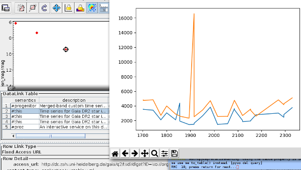
Topcat is doing datalink, and our little python script has plotted a two-color time series of RMC 18 (or so I think).
If anyone ever writes a history of the VO, the second data release of Gaia on April 25, 2018 will probably mark its coming-of-age – at least if you, like me, consider the Registry the central element of the VO. It was spectacular to view the spike of tens of Registry queries per second right around 12:00 CEST, the moment the various TAP services handing out the data made it public (with great aplomb, of course).
In GAVO's Data Center we also carry Gaia DR2 data. Our host institute, the Zentrum für Astronomie in Heidelberg, also has a dedicated Gaia server. This gives relieves us from having to be a true mirror of the upstream data release. And since the source catalog has lots and lots of columns that most users will not be using most of the time, we figured a “light” version of the source catalog might fill an interesting ecological niche: Behold gaia.dr2light on the GAVO DC TAP service, containing essentially just the basic astrometric parameters and the diagonal of the covariance matrix.
That has two advantages: Result sets with SELECT * are a lot less unwieldy (but: just don't do this with Gaia DR2), and, more importantly, a lighter table puts less load on the server. You see, conventional databases read entire rows when processing data, and having just 30% of the columns means we will be 3 times faster on I/O-bound tasks (assuming the same hardware, of course). Hence, and contrary to several other DR2-carrying sites, you can perform full sequential scans before timing out on our TAP service on gaia.dr2light. If, on the other hand, you need to do debugging or full-covariance-matrix error calculations: The full DR2 gaia_source table is available in many places in the VO. Just use the Registry.
Photometry via TAP
A piece of Gaia DR2 that's not available in this form anywhere else is the lightcurves; that's per-transit photometry in the G, BP, and RP band for about 0.5 million objects that the reduction system classified as variable. ESAC publishes these through datalink from within their gaia_source table, and what you get back is a VOTable that has the photometry in the three bands interleaved.
I figured it might be useful if that data were available in a TAP-queriable table with lightcurves in the database. And that's how gaia.dr2epochflux came into being. In there, you have three triples of arrays: the epochs (g_transit_time, bp_obs_time, and rp_obs_time), the fluxes (g_transit_flux, bp_flux, and rp_flux), and their errors (you can probably guess their names). So, to retrieve G lightcurves where available together with a gaia_source query of your liking, you could write something like:
SELECT g.*, g_transit_time, g_transit_flux
FROM gaia.dr2light AS g
LEFT OUTER JOIN gaia.dr2epochflux
USING (source_id)
WHERE ...whatever...
– the LEFT OUTER JOIN arranges things such that the g_transit_time and g_transit_flux columns simply are NULL when there are no lightcurves; with a normal (“inner”) join, rows without lightcurves would not be returned in such a query.
To give you an idea of what you can do with this, suppose you would like to discover new variable blue supergiants in the Gaia data (who knows – you might discover the precursor of the next nearby supernova!). You could start with establishing color cuts and train your favourite machine learning device on light curves of variable blue supergiants. Here's how to get (and, for simplicity, plot) time series of stars classified as blue supergiants by Simbad for which Gaia DR2 lightcurves are available, using pyvo and a little async trick:
from matplotlib import pyplot as plt
import pyvo

def main():
  simbad = pyvo.dal.TAPService(
    "http://simbad.u-strasbg.fr:80/simbad/sim-tap")
  gavodc = pyvo.dal.TAPService("http://dc.g-vo.org/tap")

  # Get blue supergiants from Simbad
  simjob = simbad.submit_job("""
    select main_id, ra, dec
    from basic
    where otype='BlueSG*'""")
  simjob.run()

  # Get lightcurves from Gaia
  try:
    simjob.wait()
    time_series = gavodc.run_sync("""
      SELECT b.*, bp_obs_time, bp_flux, rp_obs_time, rp_flux
      FROM (SELECT
         main_id, source_id, g.ra, g.dec
         FROM
        gaia.dr2light as g
         JOIN TAP_UPLOAD.t1 AS tc
         ON (0.002>DISTANCE(tc.ra, tc.dec, g.ra, g.dec))
      OFFSET 0) AS b
      JOIN gaia.dr2epochflux
      USING (source_id)
      """,
      uploads={"t1": simjob.result_uri})
  finally:
    simjob.delete()

  # Now plot one after the other
  for row in time_series.table:
    plt.plot(row["bp_obs_time"], row["bp_flux"])
    plt.plot(row["rp_obs_time"], row["rp_flux"])
    plt.show(block=False)
    raw_input("{}; press return for next...".format(row["main_id"]))
    plt.cla()

if __name__=="__main__":
  main()
If you bother to read the code, you'll notice that we transfer the Simbad result directly to the GAVO data center without first downloading it. That's fairly boring in this case, where the table is small. But if you have a narrow pipe for one reason or another and some 105 rows, passing around async result URLs is a useful trick.
In this particular case the whole thing returns just four stars, so perhaps that's not a terribly useful target for your learning machine. But this piece of code should get you started to where there's more data.
You should read the column descriptions and footnotes in the query results (or from the reference URL) – this tells you how to interpret the times and how to make magnitudes from the fluxes if you must. You probably can't hear it any more, but just in case: If you can, process fluxes rather than magnitudes from Gaia, because the errors are painful to interpret in magnitudes when the fluxes are small (try it!).
Note how the photometry data is stored in arrays in the database, and that VOTables can just transport these. The bad news is that support for manipulating arrays in ADQL is pretty much zero at this point; this means that, when you have trained your ML device, you'll probably have to still download lots and lots of light curves rather than write some elegant ADQL to do the filtering server-side. However, I'd be highly interested to work out how some tastefully chosen user defined functions might enable offloading at least a good deal of that analysis to the database. So – if you know what you'd like to do, by all means let me know. Perhaps there's something I can do for you.
Incidentally, I'll talk a bit more about ADQL arrays in a blog post coming up in a few weeks (I think). Don't miss it, subscribe to our feed).
Datalink
In the results from queries involving gaia.dr2epochflux, we also provide datalinks. These let you retrieve lightcurves that already have mags and that are more easily plotted. Perhaps more importantly, they link back to the full ESAC lightcurves that, in addition, give you a lot more debug information and are required if you want to reliably identify photometry points with the identifiers of the transits that generated them.
Datalink support in clients still is not great, but it's growing nicely. Your ideas for workflows that should be supported are (again) most welcome – and have a good chance of being adopted. So, try things out, for instance by getting the most recent TOPCAT (as of this writing) and do the following:
Open the VO/TAP dialog from the menu bar and double click the GAVO DC TAP service.
Enter:
  SELECT source_id, ra, dec,
  phot_bp_mean_mag, phot_rp_mean_mag, phot_g_mean_mag,
  g_transit_time, g_transit_flux,
  rp_obs_time, rp_flux
  FROM gaia.dr2epochflux
  JOIN gaia.dr2light
  USING (source_id)
  WHERE parallax>50

into “ADQL” text to retrieve lightcurves for the more nearby
variables (in reality, you'd have to be a bit more careful with the
distances, but you already knew that).
plot something like phot_bp_mean_mag-phot_rp_mean_mag vs. phot_g_mean_mag (and adapt the plot to fit your viewing habits).
Open the dialog for Views/Activation Actions (from the menu bar or the tool bar – same thing), check “Invoke Service”, choose “View Datalink Table”.
Whenever you click on a a point in your CMD, a window will pop up in which you can choose between the time series in the various bands, and you can pull in the data from ESAC; to load a table, select “Load Table” from the actions near the foot of the datalink table and click “Invoke”.
Yeah. It's clunky. Help us make it better with your fresh ideas for interfaces (and don't be cross with us if we have to marry them with what's technically feasible and readily generalised).
SSAP and Obscore
If you're fed up with bleeding-edge tech, the light curves are also available through good old SSAP and Obscore. To use that, just get Splat (or another SSA client, preferably with a bit of time series support). Look for a Gaia DR2 time series service (you may have to update the service list before you find it), enter (in keeping with our LBV theme) S Dor as position and hit “Lookup” followed by “Send Query”. Just click on any result to just view the time series – and then apply Splat's rich tool set to it.
Update (8.5.2018): Clusters
Here's another quick application – how about looking for variable stars in clusters? This piece of ADQL should get you started:
SELECT TOP 100
  source_id, ra, dec, parallax, g.pmra, g.pmdec,
  m.name, m.pmra AS c_pmra, m.pmde AS c_pmde,
  m.e_pm AS c_e_pm,
  1/dist AS cluster_parallax
FROM
  gaia.dr2epochflux
  JOIN gaia.dr2light AS g USING (source_id)
  JOIN mwsc.main AS m
  ON (1=CONTAINS(
    POINT(g.ra, g.dec),
    CIRCLE(m.raj2000, m.dej2000, rcluster)))
WHERE IN_UNIT(pmdec, 'deg/yr') BETWEEN m.pmde-m.e_pm*3 AND m.pmde+m.e_pm*3
– yes, you'll want to constrain pmra, too, and the distance, and properly deal with error and all. But you get simple lightcurves for free. Just add them in the SELECT clause!