Posts with the Tag Coverage:

• Crazy Shapes in TAP

  2020-09-22 Markus Demleitner

  

  A complex shape from OpenNGC: MOCs need not be convex, or simply connected, or anything.

  So far when you did spherical geometry in ADQL, you had points, circles, and polygons as data types, and you could test for intersection and containment as operations. This feature set is a bit unsatisfying because there are no (algebraic) groups in this picture: When you join or intersect two circles, the result only is a circle if one contains the other. With non-intersecting polygons, you will again not have a (simply connected) spherical polygon in the end.

  Enter MOCs (which I've mentioned a few times before on this blog): these are essentially arbitrary shapes on the sky, in practice represented through lists of pixels, cleverly done so they can be sufficiently precise and rather compact at the same time. While MOCs are powerful and surprisingly simple in practice, ADQL doesn't know about them so far, which limits quite a bit what you can do with them. Well, DaCHS would serve them since about 1.3 if you managed to push them into the database, but there were no operations you could do on them.

  Thanks to work done by credativ (who were really nice to work with), funded with some money we had left from our previous e-inf-astro project (BMBF FKZ 05A17VH2) on the pgsphere database extension, this has now changed. At least on the GAVO data center, MOCs are now essentially first-class citizens that you can create, join, and intersect within ADQL, and you can retrieve the results. All operators of DaCHS services are just a few updates away from being able to offer the same.

  So, what can you do? To follow what's below, get a sufficiently new TOPCAT (4.7 will do) and open its TAP client on http://dc.g-vo.org/tap (a.k.a. GAVO DC TAP).

  Basic MOC Operations in TAP

  First, let's make sure you can plot MOCs; run

  SELECT name, deepest_shape
  FROM openngc.shapes
  

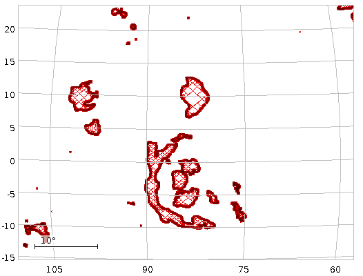
  Then do Graphics/Sky Plot, and in the window that pops up then, Layers/Add Area Control. Then select your new table in the Position tab, and finally choose deepest_shape as area (yeah, this could become a bit more automatic and probably will over time). You will then see the footprints of a few NGC objects (OpenNGC's author Mattia Verga hasn't done all yet; he certainly welcomes help on OpenNGC's version control repo), and you can move around in the plot, yielding perhaps something like Fig. 1.

  Now let's color these shapes by object class. If you look, openngc.data has an obj_type column – let's group on it:

  SELECT
    obj_type,
    shape,
    AREA(shape) AS ar
  FROM (
    SELECT obj_type, SUM(deepest_shape) AS shape
    FROM openngc.shapes
    NATURAL JOIN openngc.data
    GROUP BY obj_type) AS q
  

  (the extra subquery is a workaround necessary because the area function wants a geometry or a column reference, and ADQL doesn't allow aggregate functions – like sum – as either of these).

  In the result you will see that so far, contours for about 40 square degrees of star clusters with nebulae have been put in, but only 0.003 square degrees of stellar associations. And you can now plot by the areas covered by the various sorts of objects; in Fig. 2, I've used Subsets/Classify by Column in TOPCAT's Row Subsets to have colours indicate the different object types – a great workaround when one deals with categorial variables in TOPCAT.

  MOCs and JOINs

  Another table that already has MOCs in them is rr.stc_spatial, which has the coverage of VO resources (and is the deeper reason I've been pushing improved MOC support in pgsphere – background); this isn't available for all resources yet , but at least there are about 16000 in already. For instance, here's how to get the coverage of resources talking about planetary nebulae:

  SELECT ivoid, res_title, coverage
  FROM rr.subject_uat
    NATURAL JOIN rr.stc_spatial
    NATURAL JOIN rr.resource
  WHERE uat_concept='planetary-nebulae'
    AND AREA(coverage)<20
  

  (the rr.subject_uat table is a local extension to RegTAP that will be the subject of some future blog post; you could also use rr.res_subject, but because people still use wildly different keyword schemes – if any –, that wouldn't be as much fun). When plotted, that's the left side of Fig. 3. If you do that yourself, you will notice that the resolution here is about one degree, which is a special property of the sort of MOCs I am proposing for the Registry: They are of order 6. Resolution in MOC goes up with order, doubling with every step. Thus MOCs of order 7 have a resolution of about half a degree, MOCs of order 5 a resolution of about two degrees.

  One possible next step is fetch the intersection of each of these coverages with, say, the DFBS (cf. the post on Byurakan spectra). That would look like this:

  SELECT
    ivoid,
    res_title,
    gavo_mocintersect(coverage, dfbscoverage) as ovrlp
  FROM (
    SELECT ivoid, res_title, coverage
    FROM rr.subject_uat
    NATURAL JOIN rr.stc_spatial
    NATURAL JOIN rr.resource
    WHERE uat_concept='planetary-nebulae'
    AND AREA(coverage)<20) AS others
  CROSS JOIN (
    SELECT coverage AS dfbscoverage
    FROM rr.stc_spatial
    WHERE ivoid='ivo://org.gavo.dc/dfbsspec/q/spectra') AS dfbs
  

  (the DFBS' identifier I got with a quick query on WIRR). This uses the gavo_mocintersect user defined function (UDF), which takes two MOCs and returns a MOC of their common pixels. Which is another important part why MOCs are so cool: together with union and intersection, they form groups. It should not come as a surprise that there is also a gavo_mocunion UDF. The sum aggregate function we've used in our grouping above is (conceptually) built on that.

  

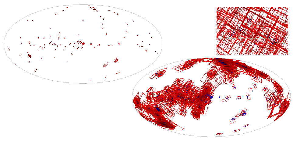
  Fig. 3: Left: The common footprint of VO resources declaring a subject of planetary-nebula (and declaring a footprint). Right bottom: Heidelberg plates intersecting this, and, in blue, level-6 intersections. Above this, an enlarged detail from this plot.

  You can also convert polygons and circles to MOCs using the (still DaCHS-only) MOC constructor. For instance, you could compute the coverage of all resources dealing with planetary nebulae, filtering against obviously over-eager ones by limiting the total area, and then match that against the coverages of images in, say, the Königstuhl plate achives HDAP. Watch this:

  SELECT
    im.*,
    gavo_mocintersect(MOC(6, im.coverage), pn_coverage) as ovrlp
  FROM (
    SELECT SUM(coverage) AS pn_coverage
    FROM rr.subject_uat
    NATURAL JOIN rr.stc_spatial
    WHERE uat_concept='planetary-nebulae'
    AND AREA(coverage)<20) AS c
  JOIN lsw.plates AS im
  ON 1=INTERSECTS(pn_coverage, MOC(6, coverage))
  

  – so, the MOC(order, geo) function should give you a MOC for other geometries. There are limits to this right now because of limitations of the underlying MOC library; in particular, non-convex polygons are not supported right now, and there are precision issue. We hope this will be rectified soon-ish when we base pgsphere's MOC operations on the CDS HEALPix library. Anyway, the result of this is plotted on the right of Fig. 3.

  Open Ends

  In case you have MOCs from the outside, you can also construct MOCs from literals, which happen to be the ASCII MOCs from the standard. This could look like this:

  SELECT TOP 1
    MOC('4/30-33 38 52 7/324-934') AS ar
  FROM tap_schema.tables
  

  For now, you cannot combine MOCs in CONTAINS and INTERSECTS expressions directly; this is mainly because in such an operation, the machine as to decide on the order of the MOC the other geometries are converted to (and computing the predicates between geometry and MOC directly is really painful). This means that if you have a local table with MOCs in a column cmoc that you want to compare against a polygon-valued column coverage in a remote table like this:

  SELECT db.* FROM
    lsw.plates AS db
    JOIN tap_upload.t6
  ON 1=CONTAINS(coverage, cmoc) -- fails!
  

  you will receive a rather scary message of the type “operator does not exist: spoly <@ smoc”. To fix it (until we've worked out how to reasonably let the computer do that), explicitly convert the polygon:

  SELECT db.* FROM
    lsw.plates AS db
    JOIN tap_upload.t6
  ON 1=CONTAINS(MOC(7, coverage), cmoc)
  

  (be stingy when choosing the order here – MOCs that already exist are fast, but making them at high order is expensive).

  Having said all that: what I've written here is bleeding-edge, and it is not standardised yet. I'd wager, though, that we will see MOCs in ADQL relatively soon, and that what we will see will not be too far from this experiment. Well: Some rough edges, I'd hope, will still be smoothed out.

  Getting This on Your Own DaCHS Installation

  If you are running a DaCHS installation, you can contribute to takeup (and if not, you can stop reading here). To do that, you need to upgrade to DaCHS's latest beta (anything newer than 2.1.4 will do) to have the ADQL extension, and, even more importantly, you need to install the postgresql-postgres package from our release repository (that's version 1.1.4 or newer; in a few weeks, getting it from Debian testing would work as well).

  You will probably not get that automatically, because if you followed our normal installation instructions, you will have a package called postgresql-11-pgsphere installed (apologies for this chaos; as ususal, every single step made sense). The upshot is that with our release repo added, sudo apt install postgresql-pgsphere should give you the new code.

  That's not quite enough, though, because you also need to acquaint the database with the new functions. This can only be done with database administrator privileges, which DaCHS by design does not possess. What DaCHS can do is figure out the commands to do that when it is called as dachs upgrade -e. Have a look at the output, and if you are satisfied it is about what to expect, just pipe it into psql as a superuser; in the default installation, dachsroot would be sufficiently privileged. That is:

  dachs upgrade -e | psql gavo   # as dachsroot
  

  If running:

  select top 1 gavo_mocunion(moc('1/3'), moc('2/9'))
  from tap_schema.tables
  

  through your TAP endpoint returns '1/3 2/9', then all is fine. For entertainment, you might also make sure that gavo_mocintersect(moc('1/3'), moc('2/13')) is 2/13 as expected, and that if you intersect with 2/3 you get back an empty string.

  So – let's bring MOCs to ADQL!

• A Grey Eminence of a Standard

  2018-10-30 Markus Demleitner

  

  Examples for extra metadata: extended column descriptions on the web pages accompanying the ARI-Gaia TAP service.

  Last friday, I've uploaded a first working draft of VODataService 1.2 to the IVOA documents repository. That's the first major step in updating a standard, and it's an invitation to everyone to have a look and comment.

  Foof, you might say, what do I care? I've not even heard of that standard.

  Well, but you've probably used it. VODataService is (among several other things) the standard that governs how a TAP service tells clients (TOPCAT, say) what tables it has and what's inside of them. So, if you see in TOPCAT that there is a column named ang_error with a unit of deg, a UCD of stat.error;pos and the meaning “1 σ confidence radius of the position”, that most likely came in a document standardised by VODataService.

  The question of what (TAP) services can tell clients about their table set is one major open point: Do we want additional metadata there? This article's image, for inspiration, shows a screenshot of extended metadata Grégory delivers to browsers on his ARI-Gaia service; among this are minima, maxima, means, standard deviations, quartiles, and fill factors (i.e., how many of the columns are NULL). He even shows histograms of the values' distributions and HEALPix maps showing how (the means of) the values vary on the sky. Another example of extended metadata could be footnotes as you will find them on many of my resources' reference URLs (example; footnotes are, unsurprisingly, near the foot of that page).

  We could define interoperable means to communicate information like this. The question is: does the added value justify the complication in implementation? This is where it would be great if you weighed in, in particular if you are a “mere” TAP user: Are there any such pieces of metadata you've always wanted to see in your TAP interfaces? Oh, and metadata of course can also be added to tables rather than columns. The current draft already lets services communicate the number of rows in each table – is there more “simple”, table-specific metadata of this sort?

  VODataService furthermore deals with several other topics; for instance, the STC in the registry business I've blogged about in February is going to be standardised here (update on this: spectral coverage is no longer in wavelength but in energy). Other changes are rather more technical in nature, like several new resource types that will improve the discovery of tables and other such resources, or a careful adjustment of some features to keep them in line with TAP evolution.

  But don't let the technicalities scare you away – just have a peek, and if you have thoughts on any of the VODataService topics: I'm just a mail away.

• DaCHS 1.2 is out

  2018-07-17 Markus Demleitner

  Today, I have released DaCHS 1.2 – somewhat belatedly perhaps, because I managed to break my collarbone, but here it is. If you've been following this blog, you already know about the headline news: the dachs start command, ADQL 2.1, and early support for STC in the registry.

  If you're not yet on DaCHS 1.1, please have a quick look at the corresponding release article. While the upgrade itself should work fine in one go even from older versions, the release notes of course apply cumulatively, and you may still have to do the dist-upgrade to 1.1.

  As usual, the generic upgrading instructions are available in the operator's guide (in short: do a dachs val ALL; apt update; apt upgrade). Since I've still encountered DaCHS installations with wrong sources.lists last April: Note again that our repository names have changed in August 2016 – we now have release and beta rather than Debian release names. So, make sure you have something like:

  deb http://vo.ari.uni-heidelberg.de/debian release main
  

  in your /etc/apt/sources.list, not something containing “stable” or the like.

  That said, here's the commented changes for 1.2:

  • New dachs start command to produce structured templates for certain service types. See Horror Vacui Begone on this blog for the full story.
  • Support for ADQL 2.1 (actually, its current proposed recommendation), including almost all of the optional parts (see Speak out on ADQL 2.1 on this blog). While not strictly necessary, it's a good idea to run dachs imp //adql after the upgrade; this will give you some nice new UDFs, in particular gavo_histogram.
  • New coverage element (with updaters) to build and declare the space-time-spectral coverage of a resource. It would be great if you could add coverage elements to your resources where it makes sense and re-publish them. This blog post tells you how to do it (you'll have to scroll down a bit).
  • There is now odbcGrammar to feed an import from another database. Essentially, you put an ODBC connection string into a file, point your sources element there, and you'll get one rawdict per tuple in a foreign database table. This might be a nice way to publish moderate-size non-postgres tables via DaCHS.
  • You can now declare associated datalink services for tables using the _associatedDatalinkSvc meta item. In particular, if you had a datalink property on SSAP services, you should migrate at some point. One advantage: Users will get the datalinks even when querying the tables through TAP. See “Integrating Datalink Services” in the reference documentation for the full story.
  • We now force matplotlib to read its configuration from /var/gavo/etc/matplotlibrc; to get a default, just run dachs init again. This is mainly to avoid uncontrolled imports of matplotlibrcs when DaCHS is run under a uid that does other things now and then.
  • DaCHS now supports VOSI 1.1; in particular, DaCHS now understands the detail hints and has per-table endpoints, so clients like TOPCAT could avoid reading the full table metadata in one go. Realistically, at least TOPCAT doesn't yet, so this is perhaps less cool than it may sound.
  • The indices generated by the ssa mixins are now a bit more sensible considering typical query modes. You probably want to run dachs imp -I on the RDs for your ssap data collections when convenient. If you have larger spectral collections, chances are many queries will be a lot faster.
  • ssapCore no longer wantonly adds preview columns. If you have previews with spectra, you probably want to add <property name="previews">auto</property> to your ssapCores. If you don't, the preview column will not be added to SSA responses (right now, few clients evaluate it, but that will hopefully change in the future).
  • You can now add a statisticsTarget property to columns; you will want this on largish tables with non-uniformly distributed values to aid the query planner; something like <property key=" statisticsTarget">10000</property> within the corresponding column element can go a long way to improve query planning (you need to run gavo imp -m on the RD after the change).
  • DaCHS's log now by default does not contain IP addresses, user agents, and referrers any more, which should mostly keep you from processing personal data and thus from having to muck around with the EU GDPR. To get back the previous behaviour, set [web]logFormat in /etc/gavo.rc to combined.
  • I fixed some utypes for obscore 1.1. These utypes are useless, so there's nothing you have to do. But then stilts taplint complains about them, and so you may want to run dachs imp -m //obscore.
  • As usual, there are many minor bug fixes and improvements (e.g., memmapping FITSes for cutout again, delimited table references in ADQL, new-style tutorial resource records, correct obscore standardId, much saner nD-arrays in VOTables).

  Well – enjoy the release, and if something goes wrong with it, be sure to let us know, preferably on the DaCHS-suppport mailing list.

Page 1 / 1