Posts with the Tag Gaia:

• At the Gaia Passivation Event

  2025-03-27 Markus Demleitner

  • 9:00
  • 9:35
  • 9:42
  • 9:45
  • 9:50
  • 9:53
  • 9:55
  • 12:00
  • 12:30
  • 13:00

  [All times in CET]

  9:00

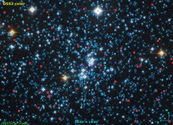
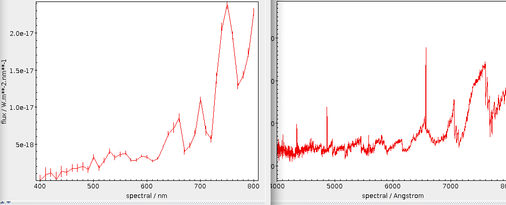
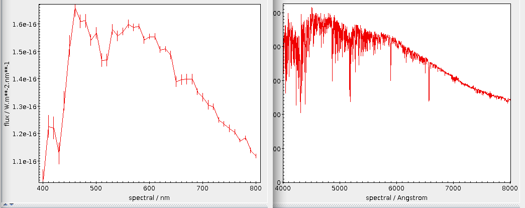
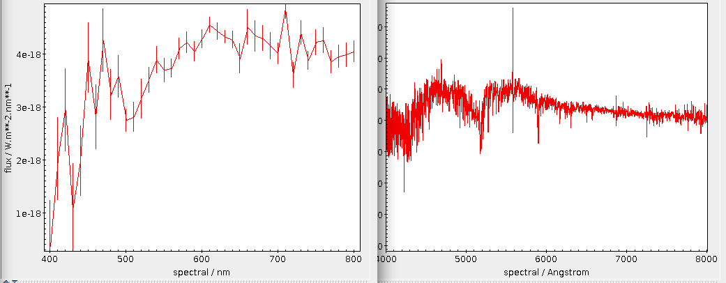
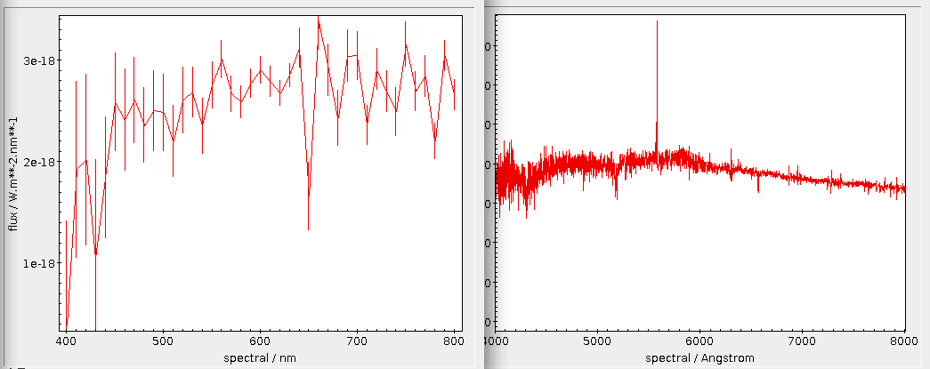
  The instrument that featured most frequently (try this) in this blog is ESA's Gaia Spacecraft that, during the past eleven years, has obtained the positions and much more (my personal favourite: the XP spectra) of about two billion objects, mostly of stars, but also of quasars, asteroids and whatever else is reasonably point-like.

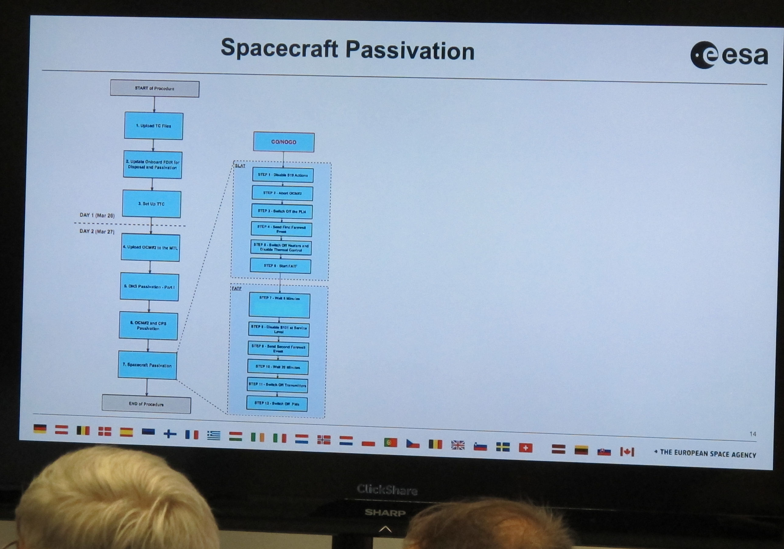
  Today, this mission comes to an end. To celebrate it – the mission, not the end, I would say –, ESA has organised a little ceremony at its operations centre in Darmstadt, just next to Heidelberg. To my serious delight, I was invited to that farewell party, and I am now listening to an overview of the passivation given by David Milligan, who used to manage spacecraft operations. This is a suprisingly involved operation, mostly because spacecraft are built to recover from all kinds of mishaps automatically and thus will normally come back on when you switch them off:

  

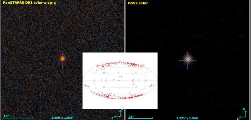
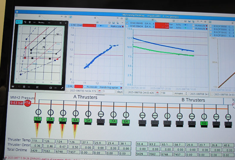
  But for now Gaia is still alive and kicking; the control screen shows four thrusters accelerating Gaia out of L2, the Lagrange point behind Earth, where it has been taking data for all these years (if you have doubts, you could check amateur images of Gaia taken while Gaia was particularly bright in the past few months; the service to collect them runs on my data centre).

  They are working the thrusters quite a bit harder than they were designed for to get to a Δv of 120 m/s (your average race car doesn't make that, but of course it takes a lot less time to accelerate, too). It is not clear yet if they will burn to the end; but even if one fails early, David explains, it is already quite unlikely that Gaia will return.

  

  9:35

  Just now the thrusters on the spacecraft have been shut down (”nominally”, as they say here, so they've reached the 120 m/s). Gaia is now on its way into a heliocentric orbit that, as the operations manager said, will bring it back to the Earth-Moon-System with chance of less than 0.25% between now and 2125. That's what much of this is about: You don't want Gaia to crash into anything else that's populating L2 (or something else near Earth, for that matter), or start randomly sending signals that might confuse other missions.

  9:42

  Gaia is now going blind. They have switched off the science computers a few minutes ago, which we could follow on the telemetry screen, and now they are switching off the CCDs, one after the other. The RP/BP CCDs, the ones that obtained my beloved XP spectra, are already off. Now the astrometry CCDs go grey (on the screen) one after the other. This feels oddly sombre.

  In a nerdy joke, they switched off the CCDs so the still active ones formed the word ”bye” for a short moment:

  

  9:45

  The geek will inherit the earth. Some nerd has programmed Gaia to send, while it is slowly winding down, an extra text message: “The cosmos is vast. So is our curiosity. Explore!”. Oh wow. Kitsch, sure, but still goosebumpy.

  9:50

  Another nerdy message: ”Signing off. 2.5B stars. countless mysteries unlocked.” Sigh.

  9:53

  Gaia is now mute. The operations manager gave a little countdown and then said „mark”. We got to see the spectrum of the signal on the ground station, and then watch it disappear. There was dead silence in the room.

  9:55

  Gaia was still listening until just now. Then they sent the shutdown command to the onboard computer, so it's deaf, too, or actually braindead. Now there is no way to revive the spacecraft short of flying there. ”This is a very emotional moment,” says someone, and while it sounds like an empty phrase, it is not right now. ”Gaia has changed astronomy forever”. No mistake. And: ”Don't be sad that it's over, be glad that it happened”.

  12:00

  Before they shut down Gaia, they stored messages from people involved with the mission in the onboard memory – and names of people somehow working on Gaia, too. And oh wow, I found my name in there, too:

  

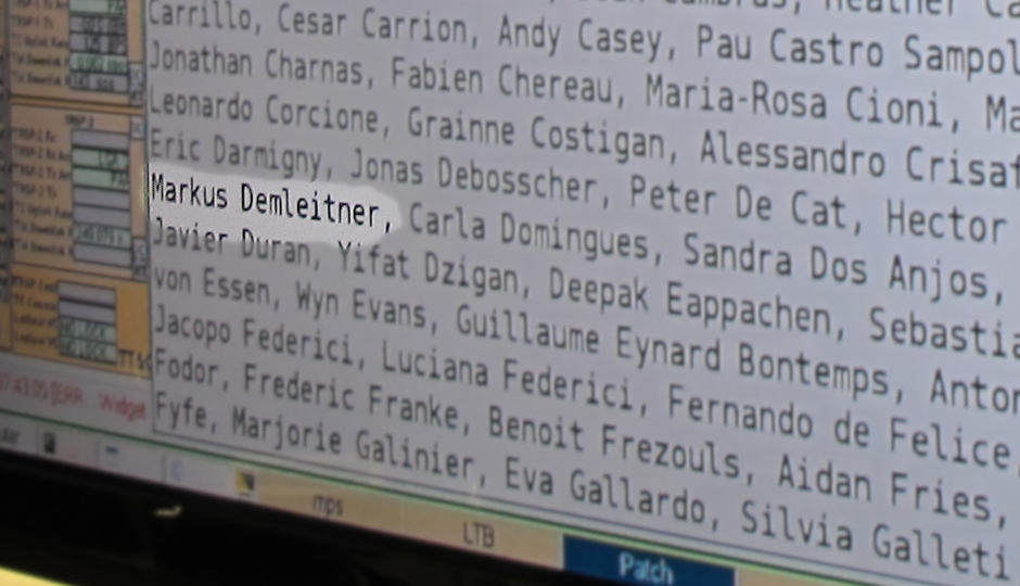
  It felt a bit odd to have my name stored aboard a spacecraft in an almost eternal heliocentric orbit.

  But on reflection: This is solid state storage, in other words, some sort of EPROM. And that means that given the radiation up there, the charges that make up the bit pattern will not live long; colleagues estimated that, with a lot of luck, this might still be readable 20 years from now, but certainly not much longer. So, no, it's not like I now share Kurt Waldheim's privilege of having something of me stored the better part of eternity.

  12:30

  Andreas Rudolph, head of operations, now gives a talk on, well, ”Gaia Operations”.

  I have already heard a few stories of the olden days while chatting to people around here. For instance, ESTEC staff is here and gave some insight views on the stray light trouble that caused quite a few sleepless nights when it was discovered during commissioning. Eventually it turned out it was because of fibres sticking out from the sunshield. Today I learned that had a long history because unfolding the sunshield actually was a hard problem during spacecraft design, and, as Andreas just reminded us, a nail-biting moment during commissioning. The things need to be rollable but stiff, and unroll reliably once in space.

  People thought of almost everything. But once they showed the sunshield to an optical engineer while debugging the problem, after a few minutes he shone the flashlight of his telephone behind the screens and conclusively demonstrated the source of the stray light.

  Space missions are incredibly hard. Even the smallest oversights can have tremendous consequences (although the mission extension after the original five years of mission time certainly helped offsetting the stray light problem).

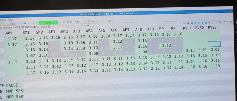
  Andreas discussed more challenges like that, in particular the still somewhat mysterious Basic Angle Variation, and finished predicting that in 2029, Gaia will next approach Earth, passing at a distance of about 10 million kilometers. I don't think it will be accessible to amateur telescopes, perhaps not even to professional ones. But let's see.

  13:00

  Gaia data processing is (and will be for another 10 years or so) performed by a large international collaboration called DPAC. DPAC is headed by Anthony Brown, and his is the last talk for today. He mentioned some of the exciting science results of the Gaia mission. Of course, that is a minute sample taken from the thousands and thousands of papers that would not exist without Gaia.

  • The tidal bridge of stars between the LMC and the SMC.
  • The discovery of 160'000 asteroids (with 5.5 years of data analysed), and their rough spectra, allowing us to group them into several classes.
  • The high-precision reference catalogue which is now in use everywhere to astrometrically calibrate astronomical images; a small pre-release of this was already in use for the navigation of the extended mission of the Pluto probe New Horizons.
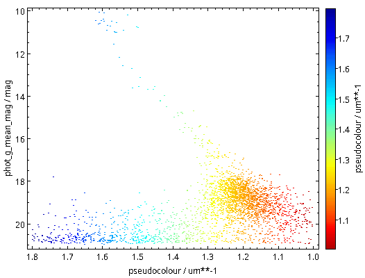
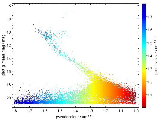
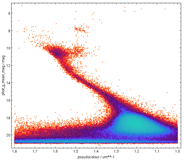
  • Finding the young stars in the (wider) solar neighbourhood by their over-luminosity in the colour-magnitude diagram, which lets you accurately map star forming regions out to a few hundred parsecs.
  • Unraveling the history of the Milky Way by reconstructing orbits of hundreds of millions of stars and identifying stellar streams (or rather, overdensities in the space of orbital elements) left over by mergers of other galaxies with the Milky Way and preserved over 10 billion years.
  • Confirming that the oldest stars in the Mikly Way are indeed in the bulge using the XP spectra, and reconstructing how the disk formed afterwards.
  • In the vertical motions of the disk stars, there is a clear signal of a recent perturbation (probably when the Sagittarius dwarf galaxy crashed through the Milky Way disk) and how there is now some sort of wave going through the disk and slowly petering out.
  • Certain white dwarfs (I think those consisting of carbon and nitrogen) show underluminosities because they form bizarre crystals in their outer regions (or so; I didn't quite get that part).
  • Thousands of star clusters newly discovered (and a few suspected star clusters debunked). One new discovery was actually hiding behind Sirius; it took space observations and very careful data reduction around bright sources to see it in the vicinity of this source overshining everything around it.
  • Quite a few binary stars having neutron stars or black holes as companions – where we are still not sure how some of these systems can even form.
  • Acceleration of the solar system: The sun orbits the centre of the Milky Way, once every about 220 Million years or so. So, it does not move linearly, but only very slightly so (“2 Angstrom/s²” acceleration, Anthony put it). Gaia's breathtaking precision let us measure that number for the first time.
  • Oh, and in DR4, we will see probably 1000s of new exoplanets in a mass-period range not well sampled so far: Giant planets in wide orbits.
  • And in DR5, there will even be limits on low-frequency gravitational waves.

  Incidentally, in the question session after Anthony's talk, the grandmaster of both Hipparcos and Gaia, Erik Høg, reminded everyone of the contributions by Russian astronomers to Gaia, among other things having proposed the architecture of the scanning CCDs. I personally have to say that I am delighted to be reminded of how science overcomes the insanities of politics and nationalism.

• Doing Large-Scale ADQL Queries

  2025-01-27 Markus Demleitner

  • Raising the Match Limit
  • Giving the Query More Time
  • Planning for Large Result Sets? Get in Contact!
  • Uniform-Length Partitions
  • Equal-Size Partitions

  You can do many interesting things with TAP and ADQL while just running queries returning a few thousand rows after a few seconds. Most examples you would find in tutorials are of that type, and when the right indexes exist on the queried tables, the scope of, let's say, casual ADQL goes far beyond toy examples.

  Actually, arranging things such that you only fetch the data you need for the analysis at hand – and that often is not much more than the couple of kilobytes that go into a plot or a regression or whatever – is a big reason why TAP and ADQL were invented in the first place.

  But there are times when the right indexes are not in place, or when you absolutely have to do something for almost everything in a large table. Database folks call that a sequential scan or seqscan for short. For larger tables (to give an order of magnitude: beyond 10⁷ rows in my data centre, but that obviously depends), this means you have to allow for longer run times. There are even times when you may need to fetch large portions of such a large table, which means you will probably run into hard match limits when there is just no way to retrieve your full result set in one go.

  This post is about ways to deal with such situations. But let me state already that having to go these paths (in particular the partitioning we will get to towards the end of the post) may be a sign that you want to re-think what you are doing, and below I am briefly giving pointers on that, too.

  Raising the Match Limit

  Most TAP services will not let you retrieve arbitrarily many rows in one go. Mine, for instance, at this point will snip results off at 20'000 rows by default, mainly to protect you and your network connection against being swamped by huge results you did not expect.

  You can, and frequently will have to (even for an all-sky level 6 HEALPix map, for instance, as that will retrieve 49'152 rows), raise that match limit. In TOPCAT, that is done through a little combo box above the query input (you can enter custom values if you want):

  

  If you are somewhat confident that you know what you are doing, there is nothing wrong with picking the maximum limit right away. On the other hand, if you are not prepared to do something sensible with, say, two million rows, then perhaps put in a smaller limit just to be sure.

  In pyVO, which we will be using in the rest of this post, this is the maxrec argument to run_sync and its sibling methods on TAPService.

  Giving the Query More Time

  When dealing with non-trivial queries on large tables, you will often also have to give the query some extra time. On my service, for instance, you only have a few seconds of CPU time when your client uses TAP's synchronous mode (by calling TAPService.run_sync method). If your query needs more time, you will have to go async. In the simplest case, all that takes is write run_async rather than run_sync (below, we will use a somewhat more involved API; find out more about this in our pyVO course).

  In async mode, you have two hours on my box at this point; this kind of time limit is, I think, fairly typical. If even that is not enough, you can ask for more time by changing the job's execution_duration parameter (before submitting it to the database engine; you cannot change the execution duration of a running job, sorry).

  Let us take the example of a colour-magnitude diagram for stars in Gaia DR3 with distances of about 300 pc according to Bailer-Jones et al (2021); to make things a bit more entertaining, we want to load the result in TOPCAT without first downloading it locally; instead, we will transmit the result's URI directly to TOPCAT[1], which means that your code does not have to parse and re-package the (potentially large) data.

  On the first reading, focus on the main function, though; the SAMP fun is for later:

  import time
  import pyvo
  
  QUERY = """
  SELECT
      source_id, phot_g_mean_mag, pseudocolour,
      pseudocolour_error, phot_g_mean_flux_over_error
  FROM gedr3dist.litewithdist
  WHERE
      r_med_photogeo between 290 and 310
      AND ruwe<1.4
      AND pseudocolour BETWEEN 1.0 AND 1.8
  """
  
  def send_table_url_to_topcat(conn, table_url):
      client_id = pyvo.samp.find_client_id(conn, "topcat")
      message = {
          "samp.mtype": "table.load.votable",
          "samp.params": {
              "url": table_url,
              "name": "TAP result",}
      }
      conn.notify(client_id, message)
  
  
  def main():
      svc = pyvo.dal.TAPService("http://dc.g-vo.org/tap")
      job = svc.submit_job(QUERY, maxrec=3000)
      try:
          job.execution_duration=10000  # that's 10000 seconds
          job.run()
          job.wait()
          assert job.phase=="COMPLETED"
  
          with pyvo.samp.connection(addr="127.0.0.1") as conn:
              send_table_url_to_topcat(conn, job.result_uri)
      finally:
          job.delete()
  
  if __name__=="__main__":
      main()
  

  As written, this will be fast thanks to maxrec=3000, and you wouldn't really have to bother with async just yet. The result looks nicely familiar, which means that in that distance range, the Bailer-Jones distances are pretty good:

  

  Now raise the match limit to 30000, and you will already need async. Here is what the result looks like:

  

  Ha! Numbers matter: at least we are seeing a nice giant branch now! And of course the dot colours do not represent the colours of the stars with the respective pseudocolour; the directions of blue and red are ok, but most of what you are seeing here will look rather ruddy in reality.

  You will not really need to change execution_duration here, nor will you need it even when setting maxrec=1000000 (or anything more, for that matter, as the full result set size is 330'545), as that ends up finishing within something like ten minutes. Incidentally, the result for the entire 300 pc shell, now as a saner density plot, looks like this:

  

  Ha! Numbers matter even more. There is now even a (to me surprisingly clear) horizontal branch in the plot.

  Planning for Large Result Sets? Get in Contact!

  Note that if you were after a global colour-magnitude diagram as the one I have just shown, you should probably do server-side aggregation (that is: compute the densities in a few hundred or thousand bins on the server and only retrieve those then) rather than load ever larger result sets and then have the aggregation be performed by TOPCAT. More generally, it usually pays to try and optimise ADQL queries that are slow and have huge result sets before fiddling with async and, even more, with partitioning.

  Most operators will be happy to help you do that; you will find some contact information in TOPCAT's service tab, for instance. In pyVO, you could use the get_contact method of the objects you get back from the Registry API[2]:

  >>> pyvo.registry.search(ivoid="ivo://org.gavo.dc/tap")[0].get_contact()
  'GAVO Data Centre Team (+49 6221 54 1837) <gavo@ari.uni-heidelberg.de>'
  

  That said: sometimes neither optimisation nor server-side aggregation will do it: You just have to pull more rows than the service's match limit. You see, most servers will not let you pull billions of rows in one go. Mine, for instance, will cap the maxrec at 16'000'000. What you need to do if you need to pull more than that is chunking up your query such that you can process the whole sky (or whatever else huge thing makes the table large) in manageable chunks. That is called partitioning.

  Uniform-Length Partitions

  To partition a table, you first need something to partition on. In database lingo, a good thing to partition on is called a primary key, typically a reasonably short string or, even better, an integer that maps injectively to the rows (i.e., not two rows have the same key). Let's keep Gaia as an example: the primary key designed for it is the source_id.

  In the simplest case, you can “uniformly” partition between 0 and the largest source_id, which you will find by querying for the maximum:

  SELECT max(source_id) FROM gaia.dr3lite
  

  This should be fast. If it is not, then there is likely no sufficiently capable index on the column you picked, and hence your choice of the primary key probably is not a good one. This would be another reason to turn to the service's contact address as above.

  In the present case, the query is fast and yields 6917528997577384320. With that number, you can write a program like this to split up your problem into N_PART sub-problems:

  import pyvo
  
  MAX_ID, N_PART = 6917528997577384320+1, 100
  partition_limits = [(MAX_ID//N_PART)*i
    for i in range(N_PART+1)]
  
  svc = pyvo.dal.TAPService("http://dc.g-vo.org/tap")
  main_query = "SELECT count(*) FROM ({part}) AS q"
  
  for lower, upper in zip(partition_limits[:-1], partition_limits[1:]):
    result = svc.run_sync(main_query.format(part=
      "SELECT * FROM gaia.dr3lite"
      "  WHERE source_id BETWEEN {} and {} ".format(lower, upper-1)))
    print(result)
  

  Exercise: Can you see why the +1 is necessary in the MAX_ID assignment?

  This range trick will obviously not work when the primary key is a string; I would probably partition by first letter(s) in that case.

  Equal-Size Partitions

  However, this is not the end of the story. Gaia's (well thought-out) enumeration scheme reflects to a large degree sky positions. So do, by the way, the IAU conventions for object designations. Since most astronomical objects are distributed highly unevenly on the sky, creating partitions with of equal size in identifier space will yield chunks of dramatically different (a factor of 100 is not uncommon) sizes in all-sky surveys.

  In the rather common event that you have a use case in which you need a guaranteed maximum result size per partition, you will therefore have to use two passes, first figuring out the distribution of objects and then computing the desired partition from that.

  Here is an example for how one might go about this:

  from astropy import table
  import pyvo
  
  MAX_ID, ROW_TARGET = 6917528997577384320+1, 10000000
  
  ENDPOINT = "http://dc.g-vo.org/tap"
  
  # the 10000 is just the number of bins to use; make it too small, and
  # your inital bins may already overflow ROW_TARGET
  ID_DIVISOR = MAX_ID/10000
  
  DISTRIBUTION_QUERY = f"""
  select round(source_id/{ID_DIVISOR}) as bin, count(*) as ct
  from gaia.dr3lite
  group by bin
  """
  
  
  def get_bin_sizes():
    """returns a ordered sequence of (bin_center, num_objects) rows.
    """
    # since the partitioning query already is expensive, cache it,
    # and use the cache if it's there.
    try:
      with open("partitions.vot", "rb") as f:
        tbl = table.Table.read(f)
    except IOError:
      # Fetch from source; takes about 1 hour
      print("Fetching partitions from source; this will take a while"
        " (provide partitions.vot to avoid re-querying)")
      svc = pyvo.dal.TAPService(ENDPOINT)
      res = svc.run_async(DISTRIBUTION_QUERY, maxrec=1000000)
      tbl = res.table
      with open("partitions.vot", "wb") as f:
        tbl.write(output=f, format="votable")
  
    res = [(row["bin"], row["ct"]) for row in tbl]
    res.sort()
    return res
  
  
  def get_partition_limits(bin_sizes):
    """returns a list of limits of source_id ranges exhausting the whole
    catalogue.
  
    bin_sizes is what get_bin_sizes returns (and it must be sorted by
    bin center).
    """
    limits, cur_count = [0], 0
    for bin_center, bin_count in bin_sizes:
      if cur_count+bin_count>MAX_ROWS:
        limits.append(int(bin_center*ID_DIVISOR-ID_DIVISOR/2))
        cur_count = 0
      cur_count += bin_count
    limits.append(MAX_ID)
    return limits
  
  
  def get_data_for(svc, query, low, high):
    """returns a TAP result for the (simple) query in the partition
    between low and high.
  
    query needs to query the ``sample`` table.
    """
    job = svc.submit_job("WITH sample AS "
      "(SELECT * FROM gaia.dr3lite"
      "  WHERE source_id BETWEEN {} and {}) ".format(lower, upper-1)
      +query, maxrec=ROW_TARGET)
    try:
      job.run()
      job.wait()
      return job.fetch_result()
    finally:
      job.delete()
  
  
  def main():
    svc = pyvo.dal.TAPService(ENDPOINT)
    limits = get_partition_limits(get_bin_sizes())
    for ct, (low, high) in enumerate(zip(limits[:-1], limits[1:])):
      print("{}/{}".format(ct, len(limits)))
      res = get_data_for(svc, <a query over a table sample>, low, high-1)
      # do your thing here
  

  But let me stress again: If you think you need partitioning, you are probably doing it wrong. One last time: If in any sort of doubt, try the services' contact addresses.

  [1]

  Of course, if you are doing long-running queries, you probably will postpone the deletion of the service until you are sure you have the result wherever you want it. Me, I'd probably print the result URL (for when something goes wrong on SAMP or in TOPCAT) and a curl command line to delete the job when done. Oh, and perhaps a reminder that one ought to execute the curl command line once the data is saved.

  [2]

  Exposing the contact information in the service objects themselves would be a nice little project if you are looking for contributions you could make to pyVO; you would probably do a natural join between the rr.interface and the rr.res_role tables and thus go from the access URL (you generally don't have the ivoid in pyVO service objects) to the contact role.

• Making Custom Indexes for astrometry.net

  2023-07-26 Markus Demleitner

  • Custom Indexes for Targeted Observations
  • Custom Indexes for Ancient Observations
  • Custom Indexes: Full-sky and Deep

  When you have an image or a scan of a photographic plate, you usually only have a vague idea of what position the telescope actually was pointed at. Furnishing the image with (more or less) precise information about what pixel corresponds to what sky position is called astrometric calibration. For a while now, arguably the simplest option to do astrometric calibration has been a package called astrometry.net. The eponymous web page has been experiencing… um… operational problems lately, but thanks to the Debian astronomy team, there is a nice package for it in Debian.

  However, just running apt install astrometry.net will not give you a working setup. Astrometry.net in addition needs an “index”, files that map star patterns (“quads“, in astrometry.net jargon) to positions. Debian comes with two pre-made sets of indexes at the moment (see apt search astrometry-data): those based on the Tycho 2 catalogue, and those based on 2MASS.

  For the index based on Tycho 2, you will find packages astrometry-data-tycho2-10-19, astrometry-data-tycho2-09, astrometry-data-tycho2-08, astrometry-data-tycho2-07[1]. The numbers in there (“scale numbers”) define the size of images the index is good for: 19 means “a major part of the sky”, 10 is “about a degree”, 8 “about half a degree”. Indexes for large images only have a few bright stars and hence are rather compact, which is why 10 though 19 fit into one package, whereas astrometry-data-tycho2-07-littleendian weighs in at 141 MB, and indexes at scale number 0 (suitable for images of a few arcminutes) take dozens of Gigabytes if they are for the whole sky.

  So, when you do astrometric calibration, consider the size of your images first and then decide which scale number is sensible for you. It is usually a good idea to try the neighbouring scale numbers, too.

  You can then feed these to your calibration routine. If you are running DaCHS, you will probably want to use the AnetHeaderProcessor, where you give the names of the indexes in the sp_indices; you also have to say where to find the indexes, as in:

  from gavo import api
  
  class MyObsCalibrator(api.AnetHeaderProcessor):
    indexPath = "/usr/share/astrometry"
    sp_indices = ["index-tycho2-09*.fits",
      "index-tycho2-10*.fits",
      "index-tycho2-11*.fits",]
  

  This would be suitable for images that cover about a degree on the sky.

  Custom Indexes for Targeted Observations

  The Tycho catalogue starts becoming severely incomplete below m_V ≈ 11, and since astrometry.net needs a few stars on an image to be able to calibrate it, you cannot use it to calibrate images smaller than a few tens of arcminutes (depending on where you look, of course). If you have smaller images, there are the 2MASS-based indexes; but the bluer your images are, the worse 2MASS as an infrared survey will do, and in addition, having the giant indexes is a big waste of storage and compute resources when you know your images are on a rather small part of the sky.

  In such a situation, you will save a lot of CPU and possibly even improve your astrometry if you create a custom index for your specific data. For instance, assume you have images sized about 10 arcminutes, and the observation programme covers a reasonably small set of objects (as long as it's of order a few hundred, a custom index certainly will be a good deal). You could then make your index based on Gaia positions and photometry like this:

  """
  Create an index for astrometry.net and a few small fields based on Gaia.
  
  Be sure to adapt this for your use case; for instance, if what your are
  calibrating will be from only a part of the sky, pick specific healpixes
  (perhaps on a different level; below, we're using level 5).  Also consider
  changing the target epoch, the photometry, or the magnitude limit.
  
  This script takes the sample positions from a text file; have
  space-separated pairs of ra and dec in targets.txt.
  """
  
  import os
  import subprocess
  
  from astropy.table import Table
  import pyvo
  
  # 0 is for images of about two arcminutes, 10 for about degree, 12 for two
  # degrees, etc.
  SIZE_PRESET = 1
  
  # The typical radius of your images in degrees (this is the size of our cone
  # searches, so cut some slack); this needs to be changed in unison with
  # SIZE_PRESET
  IMAGE_RADIUS = 1/10.
  
  
  def get_target_table():
      """must return an astropy table with columns ra and dec in degrees.
  
      (of course, if you have your data in a proper format with actual metadata,
      you don't need any of the ugly magic).
      """
      targets = Table.read("targets.txt", format="ascii")
      targets["col1"].name, targets["col2"].name = "ra", "dec"
      targets["ra"].meta = {"ucd": "pos.eq.ra;meta.main"}
      targets["dec"].meta = {"ucd": "pos.eq.dec;meta.main"}
      return targets
  
  
  def main():
      tap_service = pyvo.dal.TAPService("http://dc.g-vo.org/tap")
      res = tap_service.run_async(f"""
          SELECT g.ra as RA, g.dec as DEC, phot_g_mean_mag as MAG
          FROM gaia.dr3lite AS g
          JOIN TAP_UPLOAD.t1 as mine
              ON DISTANCE(mine.ra, mine.dec, g.ra, g.dec)<{IMAGE_RADIUS}""",
        uploads={"t1": get_target_table()})
  
      cat_file = "basic-cat.fits"
      res.to_table().write(cat_file, format="fits", overwrite=True)
  
      try:
          subprocess.run(["build-astrometry-index", "-i", cat_file,
              "-o", f"./index-custom-{SIZE_PRESET:02d}.fits",
              "-P", str(SIZE_PRESET), "-S", "MAG"])
      finally:
          os.unlink(cat_file)
  
  
  if __name__=="__main__":
      main()
  

  This writes a single file, index-custom-01.fits (in this case).

  If you read your positions from something else than the simple ASCII file I'm assuming here: Be sure to annotate the columns containing RA and Dec with the proper UCDs as shown here. That makes DaCHS (and perhaps other TAP services, too) create the right hints for the database, speeding up things tremendously.

  You can of course change the ADQL query; it might, for instance, help to replace the G magnitudes with RP or BP ones, or you could use a different catalogue than Gaia. Just make sure the FITS table that is written to basic-cat.fits has exactly the columns RA, DEC, and MAG.

  In DaCHS, I tend to keep scripts like the one above in a subdirectory of the resdir called custom-index, and then in the calibration script I write:

  from gavo import api
  
  RD = api.getRD("myres/q")
  
  class MyObsCalibrator(api.AnetHeaderProcessor):
    indexPath = RD.resdir
    sp_indices = ["custom-index/index-custom-01.fits"]
  

  Custom Indexes for Ancient Observations

  On the other hand, if you have oldish images not going terribly deep, you may want to tailor an index for about the epoch the images were taken at. Many bright stars have a proper motion large enough to matter over a century, and so doing epoch propagation (in this case with the ivo_epoch_prop user defined function, which is not available everywhere) is probably a good idea. The following script computes three full-sky indexes with quads around the desired size; note how you can set the limiting magnitude and the size preset:

  """
  Create a full-sky index for bright stars and astrometry.net based on Gaia.
  
  This only works for rather bright stars because the Gaia service will refuse
  to server more than ~1e7 objects.
  
  Make sure to choose SIZE_PRESET to your use case (19 means 30 deg,
  10 about a degree, two preset steps are about a factor two in scale).
  """
  
  import os
  import subprocess
  
  import pyvo
  
  # see the module docstring
  SIZE_PRESET = 12
  
  # ignore stars fainter than this; you can't go below 14 all-sky with Gaia
  # and the GAVO DC server
  MAX_MAG = 12
  
  # Epoch to transform the stars to
  TARGET_EPOCH = 1910
  
  
  def main():
      tap_service = pyvo.dal.TAPService("http://dc.g-vo.org/tap")
      res = tap_service.run_async(f"""
          SELECT pos[1] as RA, pos[2] as DEC, mag as MAG
          FROM (
              SELECT phot_bp_mean_mag AS mag,
                  ivo_epoch_prop(ra, dec, parallax,
                      pmra, pmdec, radial_velocity, 2016, {TARGET_EPOCH}) as pos
              FROM gaia.dr3lite
            WHERE phot_bp_mean_mag<{MAX_MAG}) AS q""")
  
      cat_file = "current.fits"
      res.to_table().write(cat_file, format="fits", overwrite=True)
  
      try:
          for size_preset in range(SIZE_PRESET-1, SIZE_PRESET+2):
              subprocess.run(["build-astrometry-index", "-i", cat_file,
                  "-o", f"./index-custom-{size_preset:02d}.fits",
                  "-P", str(size_preset), "-S", "MAG"])
      finally:
          os.unlink(cat_file)
  
  
  if __name__=="__main__":
      main()
  

  With this and my custom-index directory, your DaCHS header processor could say:

  from gavo import api
  
  RD = api.getRD("myres/q")
  
  class MyObsCalibrator(api.AnetHeaderProcessor):
    indexPath = RD.resdir
    sp_indices = ["custom-index/index-custom-*.fits"]
  

  Custom Indexes: Full-sky and Deep

  I have covered the cases “deep and spotty” and “shallow and full-sky“. The case “deep and full-sky“ is a bit more involved because it still lies in the realm of big data, which always requires extra tricks. In this case, that would be retrieving the basic catalogue in parts – for instance, by HEALPix – and at the same time splitting the index up between HEALPixes, too. This does not require great magic, but it does require a bit of non-trivial bookkeeping, and hence I will only write about it if someone actually needs it – if that's you, please write in.

  [1]	You will also find that each of these exist in a littleendian and bigendian flavours; ignore these, your machine will pick what it needs when you install the packages without tags.

• Gaia DR3 XP Spectra: All Sampled

  2022-09-06 Markus Demleitner

  

  Around this time of the year on the northern hemisphere, you can spot the h and χ Persei double star cluster with the naked eye. One part of it, NGC 884 is shown here with LAMOST DR6 low resolution spectra (red squares) and Gaia DR3 XP spectra (blue crosses) overplotted. Given that LAMOST has already been one of the largest collections of spectra on the planet, you can see that there is really a lot of those XP spectra.

  When Gaia DR3 was released in June, I was somewhat disappointed when I realised what it is that they delivered as the BP/RP (or XP for short) spectra. You see, I had expected to see something rather similar to what I have in DFBS: structurally, arrays of a few dozen spectral points, mapping wavelengths to some sort of measure of the flux.

  What really came were, mainly, “continuous spectra“, that is coefficients of Gauss-Hermite polynomials. You can fetch them from the gaiadr3.xp_continuous_mean_spectrum table at the ARI-Gaia TAP service; the blue part of the spectrum of the star DR3 4295806720 looks like this in there:

  102.93398893929992, -12.336921213781045, -2.668856168170544, -0.12631176306793765, -0.9347021092539146, 0.05636787290132809, [...]

  No common spectral client can plot this. The Gaia DPAC has helpfully provided a Python library called GaiaXPy to turn these into “proper” spectra. Shortly after the data release, my plan has thus been to turn all these spectra into their “sampled” form using GaiaXPy and then re-publish them, both through SSAP for ad-hoc discovery and through TAP for (potentially) global analysis.

  Alas, for objects too faint to make it into DR3's xp_sampled_mean_spectrum table (that's 35 million spectra already turned to wavelength-flux pairs by DPAC), the spectra generated in this way looked fairly awful, with lots of very artificial-looking wiggles (“ringing”, if you will). After a bit of deliberation, I realised that when the errors are given on the Hermite coefficients, once you compute the samples, these errors will be liberally distributed among the output samples. In other words, the error on the samples will be grossly correlated over arbitrary distances; at least I am fairly helpless when trying to separate signal from artefact in these beasts.

  Bummer. Well, fortunately, Rene Andrae from “up the mountain” (i.e., the MPI for Astronomy) has worked out a reasonably elegant way to get more conventional spectra understandable to mere humans. Basically, you compute n distinct “realisations” of the error model given by the table of the continuous spectra and average over them. The more samples you take, the less correlated your spectral points and their errors will be and the less confusing the signal will be. The service docs for gaia/s3 give the math.

  Doing this on more than 200 million spectra is quite an effort, though, and so after some experimentation I decided to settle on 10 realisations per spectrum and have relatively wide bins (10 nm) over just the optical part of the spectrum (400 through 800 nm). The BP and RP bandpaths are a bit wider, and there is probably signal blotted out by the wide bins; I will probably be addressing this for DR4, except if these spectra become the smash hit they deserve to be.

  The result of this procedure is now available through an SSAP service that should show up in the VO Registry by the time the first of you read this; the Aladin image above gives you an impression of the density of results here – and don't forget: the spectra with the blue crosses are all reasonably well flux-calibrated.

  The data is also available on the TAP service http://dc.g-vo.org/tap, which opens up many interesting possibilities. Let me mention two here.

  Comparison with LAMOST

  I was rather nervous whether what I had done resulted in anything that bore even a fleeting resemblance to reality, and so about the first thing I tried was to compare my new data with what LAMOST has.

  That is a nice exercise for TAP and ADQL. Let's first match spectra from the two surveys, which luckily are on the same server, saving us some cross-server uploads. I am selecting a minimum of data, just the position and the two access URLs, and I let DaCHS' MAXREC kick in so I'm just retrieving 20000 of the millions of result records:

  SELECT a.ssa_location, a.accref, b.accref
  FROM
    gdr3spec.ssameta AS a
    JOIN lamost6.ssa_lrs AS b
    ON DISTANCE(a.ssa_location, b.ssa_location)<0.001
  

  (this is using the DISTANCE(.,.)<radius idiom that we will be migrating towards in ADQL 2.1 instead of the dreaded 1=CONTAINS(POINT, CIRCLE) thing everyone has loathed in ADQL 2.0).

  Using the nifty activation actions, you can now tell TOPCAT to open the two spectra next to each other when you click on a row or a point in a sky plot. To reproduce,

  1. Make a sky plot. TOPCAT doesn't yet pick up the POINT in ssa_location, so you have to configure the Lon and Lat fields yourself to ssa_location[0] and ssa_location[1].
  2. Open the activation actions, either from the button bar or from the Views menu.
  3. In there, select Plot Table, make sure it says accref in Table Location and then check Plot Table in the Actions pane. When you now click on a point in the sky plot, you should see a spectrum pop up, except it is plotted with dots, which most people consider inappropriate for spectra. Use the Form tab in the plot window to style it a bit more spectrum-like (I recommend looking into Line and XYError).
  4. But how do you now add the LAMOST plot? I don't think TOPCAT's activation actions let you plot right into the plane plot you just configured. But you can add a second Plot Table action from the Actions menu in the window with the activation actions. As before, configure this new item, except this one needs to plot accref_ (which is what DaCHS has called the access reference for LAMOST to keep the names unique).
  5. As for Gaia, configure to plot to look good as a spectrum. In order to make the two spectra optically comparable, under Axes set the range to 4000 to 8000 Angstrom manually here.

  You can now click on points in your sky plot and, after a second or so, see the corresponding spectra next to each other (if you place the two plot windows that way).

  If you try this, you will (hopefully) see that major features of spectra are nicely reproduced, such as with these, I guess, molecular bands:

  

  As you probably have guessed, the extremely low-resolution Gaia XP spectrum is left, LAMOST's (somewhat higher-resolution) low-resolution spectrum is right:

  This also works with absorption in the blue, as in this example:

  

  In case of doubt, I have to say I'd probably trust Gaia's calibration around 400 nm better than LAMOST's. But that's mere guesswork.

  For fainter objects, you will see remnants of the systematic wiggles from the Hermite polynomials:

  

  Anyway, if you keep an eye on the errors, you can probably even work with spectra from the fainter objects:

  

  Mass Retrieval of Spectra

  One nice thing about the short spectra is that you can fetch many of them in one go and in very little time. For instance, to retrieve particularly red objects from the Gaia catalogue of Nearby Stars (also on the GAVO server) with spectra, say:

  SELECT
    source_id, ra, dec, parallax, phot_g_mean_mag,
    phot_bp_mean_mag, phot_rp_mean_mag, ruwe, adoptedrv,
    flux, flux_error
  FROM gcns.main
  JOIN gdr3spec.spectra
  USING (source_id)
  WHERE phot_rp_mean_mag<phot_bp_mean_mag-4
  

  [in case you wonder how I quickly got the column names enumerated here: do control-clicks into the Columns pane in TOCPAT's TAP window and then use the Cols button]. For when you do not have Gaia DR3 source_id-s in your source table, there is also gdr3spec.withpos against which you can do more conventional positional crossmatches.

  Within a few seconds, you can retrieve more than 4000 spectra in this way. You can now do whatever analysis you want on these spectra. Or, well, just plot them. The following procedure for that later task uses TOPCAT features only available in the next release, due before mid-October[1].

  First, make a colour-magnitude diagram (CMD) from this table as usual (e.g., BP-RP vs G). Then, open another plane plot and

  1. Layers → Add XYArray Control
  2. Configure the XYArray to plot from the table you just fetched, have nothing in X Values[2] and flux in Y Values.
  3. Under Axes, configure Y Log in order to better show the 4253 spectra at one time.
  4. Throw away or at least uncheck all other layers in the plot.
  5. In order to let TOPCAT highlight the spectrum of the activated source, in the Subsets pane check the Activated subset (that's the bleeding-edge functionality you will not have in older TOPCATs) and give it a sufficiently bright colour.

  With that, you can now click around in your CMD and immediately see that source's spectrum in the context of all the others, like this:

  

  These spectra have also inspired me to design and implement a vector extension for ADQL, which lets you do even more interesting things with these spectra. More on this… soon.

  [1]	The Activated subset is only available in TOPCAT versions later than 4.8-7 (released in October 2022).

  [2]

  These should be the spectral points; DaCHS does not deliver them with this query because I am a coward. I think I will find my courage relatively soon and then fix this. Once that has happened, you can select param$spectral as X values. [Update: Mark Taylor remarks that by writing sequence(41, 400, 10) in bleeding-edge TOPCATs and add(multiply(10,sequence(41)),400) before that, you can add a proper spectral axis until then]

• The Loneliest Star in the Sky

  2021-01-20 Markus Demleitner

  

  The loneliest star in the sky on the left, and on the right a somewhat more lonelier one (it's explained in the text). The inset shows the distribution of the 500 loneliest stars on the whole sky in Galactic coordinates.

  In early December, the object catalogue of Gaia's data release 3 was published (“eDR3“), and I've been busy in various ways on this data off and on since then – see, for instance, the The Case of the disappearing bits on this blog.

  One of the things I have missed when advising people on projects with previous Gaia data releases is a table that, for every object, gives the nearest neighbour. And so for this release I've created it and christened it, perhaps just a bit over-grandiosely, “Gaia eDR3 Autocorrelation”. Technically, it is just a long (1811709771 rows, to be precise) list of pairs of Gaia eDR3 source ids, the ids of their nearest neighbour, and a spherical distance between.

  This kind of data is useful for many applications, mostly when looking for objects that are close together or (more often) things that fail for such close pairs for a wide variety of reasons. I have taken some pains to not only have close neighbours, though, because sometimes you may want specifically objects far away from others.

  As in the case of this article's featured image: The loneliest star in the sky (as seen by Gaia, that is) is eDR3 6049144983226879232, which is 4.3 arcminutes from its neighbour, 6049144021153793024, which in turn is the second-loneliest star in the sky. They are, perhaps a bit surprisingly, in Ophiuchus (and thus fairly close to the Milky Way plane), and (probably) only about 150 parsec from Earth. Doesn't sound too lonely, hm? Turns out: these stars are lonely because dust clouds blot out all their neighbours.

  Rank three is in another dust cloud, this time in Taurus, and so it continues in low Galactic latitude to rank 8 (4402975278134691456) at Galactic latitude 36.79 degrees; visualising the thing, it turns out it's again in a dark cloud. What about rank 23 at 83.92 Galactic (3954600105683842048)? That's probably bona-fide, or at least it doesn't look very dusty in the either DSS or PanSTARRS. Coryn (see below) estimates it's about 1100 parsec away. More than 1 kpc above the galactic disk: that's more what I had expected for lonely stars.

  Looking at the whole distribution of the 500 loneliest stars (inset above), things return a bit more to what I had expected: Most of them are around the galactic poles, where the stellar density is low.

  So: How did I find these objects? Here's the ADQL query I've used:

  SELECT TOP 500
    ra, dec, source_id, phot_g_mean_mag, ruwe,
    r_med_photogeo,
    partner_id, dist,
    COORD2(gavo_transform('ICRS', 'GALACTIC',
      point(ra, dec))) AS glat
  FROM
    gedr3dist.litewithdist
    NATURAL JOIN gedr3auto.main
  ORDER BY dist DESC
  

  – run this on the TAP server at http://dc.g-vo.org/tap (don't be shy, it's a cheap query).

  Most of this should be familiar to you if you've worked through the first pages of ADQL course. There's two ADQL things I'd like to advertise while I have your attention:

  1. NATURAL JOIN is like a JOIN USING, except that the database auto-selects what column(s) to join on by matching the columns that have the same name. This is a convenient way to join tables designed to be joined (as they are here). And it probably won't work at all if the tables haven't been designed for that.
  2. The messy stuff with GALACTIC in it. Coordinate transformations had a bad start in ADQL; the original designers hoped they could hide much of this; and it's rarely a good idea in science tools to hide complexity essentially everyone has to deal with. To get back on track in this field, DaCHS servers since about version 1.4 have been offering a user defined function gavo_transfrom that can transform (within reason) between a number of popular reference frames. You will find more on it in the server's capabilities (in TOPCAT: the “service” tab). What is happening in the query is: I'm making a Point out of the RA and Dec given in the catalogue, tell the transform function it's in ICRS and ask it to make Galactic coordinates from it, and then take the second element of the result: the latitude.

  And what about the gedr3dist.litewithdist table? That doesn't look a lot like the gaiaedr3.gaiasource we're supposed to query for eDR3?

  Well, as for DR2, I'm again only carrying a “lite” version of the Gaia catalogue in GAVO's Heidelberg data center, stripped down to the columns you absolutely cannot live without even for the most gung-ho science; it's called gaia.edr3lite.

  But then my impression is that almost everyone wants distances and then hacks something to make Gaia's parallax work for them. That's a bad idea as the SNR goes down to levels very common in the Gaia result catalogue (see 2020arXiv201205220B if you don't take my word for it). Hence, I'm offering a pre-joined view (a virtual table, if you will) with the carefully estimated distances from Coryn Bailer-Jones, and that's this gedr3dist.litewithdist. Whenever you're doing something with eDR3 and distances, this is where I'd point you first.

  Oh, and I should be mentioning that, of course, I figured out what is in dust clouds and what is not with TOPCAT and Aladin as in our tutorial TOPCAT and Aladin working together (which needs a bit of an update, but you'll figure it out).

  There's a lot more fun to be had with this (depending on what you find fun in). What about finding the 10 arcsec-pairs with the least different luminosities (which might actually be useful for testing some optics)? Try this:

  SELECT TOP 300
    a.source_id, partner_id, dist,
    a.phot_g_mean_mag AS source_mag,
    b.phot_g_mean_mag AS partner_mag,
    abs(a.phot_g_mean_mag-b.phot_g_mean_mag) AS magdiff
  FROM gedr3auto.main
    NATURAL JOIN gaia.edr3lite AS a
    JOIN gaia.edr3lite AS b
      ON (partner_id=b.source_id)
  WHERE
    dist BETWEEN 9.999/3600 AND 10.001/3600
    AND a.phot_g_mean_mag IS NOT NULL
    AND b.phot_g_mean_mag IS NOT NULL
  ORDER BY magdiff ASC
  

  – this one takes a bit longer, as there's many 10 arcsec-pairs in eDR3; the query above looks at 84690 of them. Of course, this only returns really faint pairs, and given the errors stars that weak have they're probably not all that equal-luminosity as that. But fixing all that is left as an exercise to the reader. Given there's the RP and BP magnitude columns, what about looking for the most colourful pair with a given separation?

  Acknowledgement: I couldn't have coolly mumbled about Ophiuchus or Taurus without the SCS service ivo://cds.vizier/vi/42 (”Identification of a Constellation From Position, Roman 1982”).

  Update [2021-02-05]: I discovered an extra twist to this story: Voyager 1 is currently flying towards Ophiuchus (or so Wikipedia claims). With an industrial size package of artistic licence you could say: It's coming to keep the loneliest star company. But of course: by the time Voyager will be 150 pc from earth, eDR3 6049144983226879232 will quite certainly have left Ophiuchus (and Voyager will be in a completely different part of our sky, that wouldn't look familar to us at all) – so, I'm afraid apart from a nice conincidence in this very moment (galactically speaking), this whole thing won't be Hollywood material.

Page 1 / 2 »