Posts with the Tag stilts:

  • Requirements and Validators

    Content Warning: this is mainly VO lore. I am not claiming any immediate applicability to the use or publication of astronomical data.

    This morning, I set out to reply to a mail by Mark Taylor and noticed after a while that I was writing a philosophical piece on how to write standards – and how not to – that I may want to refer to again later. So, I'll make this a blog post.

    The story started when the excellent stilts taplint during my monthly validation routine produced an error when exercising my data centre's TAP endpoint:

    I-OBS-QSUB-5 Submitting query: SELECT TOP 1 obs_id FROM ivoa.ObsCore WHERE obs_id IS NULL
    E-OBS-QERR-1 TAP query failed [Service error: "Field query: Query timed out (took too long).
    

    What happened is that stilts tried to ascertain that all rows in my obscore table satisfy the standard's requirement that the obs_id column is non-NULL (see page 20). This made Postgres – the database system actually executing the queries – run what is known as a sequential scan through the tables involved in obscore; the reason underlying this bad judgement is a bit involved and has to do with the fact that in DaCHS, ivoa.obscore is a view composed of many tables. I will spare you the details, but the net effect of that is that it is not easy to tell Postgres that rows with obs_id NULL, if they exist at all, will be few and far between.

    By now, the number of data sets in my obscore table approaches 100'000'000, and fetching all that data simply takes time, more time than a synchronous query has on my site[1].

    Granted, I could fix that by adding indexes on the columns involved, but since these come from several dozen tables, that would be quite a bit of work for both me and the computer. Is that work worth it? Well, it certainly is if otherwise I'm breaking the standard, but since it is a serious amount of work, I am tempted to wonder: does the requirement actually make sense? And this leads to the question:

    Why do we require things in standards?

    In the end, there is just one reason to require something in a standard: Without the requirement, something important breaks. When one thinks about this a bit more deeply, one can distinguish two somewhat finer classes of requirements.

    (a) “Internal requirements“. These are rules imposed so machines can do their job. The most obvious examples here are requirements on how to write things. For instance, if a client writes an interval as lower/upper and the service expects lower upper, it just won't work. Hence, a standard has to say “The separator in intervals MUST be whitespace” (or whatever).

    There are more subtle requirements in that department. For instance, many tables need a primary key because other tables may want to refer to them. For Obscore, this becomes relevant just about now, when we think about having extensions for it. Those would add specific metadata for, say, radio or gamma observations. We will probably create them by adding per-extension tables holding a foreign key into ivoa.obscore. This is nice because then you can write something like:

    SELECT ...
    FROM ivoa.obscore
    JOIN ivoa.obs_visibility
      USING (obs_publisher_did)
    WHERE (some visiblity-specific constraint)
    

    – and almost everything just works without further thought or effort: No plethora of columns that are NULL in ivoa.obscore for anything that is not a visibility, and no manual filtering out of non-visibilities either: JOIN does it all nicely for you. Isn't relational algebra great?

    But this only is possible if obs_publisher_did (well: it's not certain yet whether that actually will be obscore's designated primary key, but bear with me there) really is non-NULL, and if there are no two rows with the same publisher DID (which are the general criteria to make something a primary key in a relation). Hence, these two constraints are something we simply MUST (pun intended) require.

    (b) “Functional requirements”. These are requirements resulting from considerations of the use of the standard. I have just encountered a nice example when working on LineTAP, a future standard on how to access data about spectral lines. An important use case there is that the client displays the lines on top of a spectrum, and it will want to put something next to the lines so the user has at least a first indication just what would cause the line to show up. That it can only do if the service provides it with a plausible label – asking clients to invent a label based on the data it has is likely to produce very unsatifying results, as no machine is smart enough to figure out nice, idiomatic strings like „21 cm HI“ or „Hα“. Hence, we simply have to require that each row in such a LineTAP table has a title (technically: the corresponding column has a non-NULL constraint).

    Going back to the obs_id example, it does not seem there is a strong case to invoke either (a) or (b) – since the column explicitly has no uniqueness requirement, it will not work as a primary key, and users will probably only want to use it for “grouped” data, where multiple artefacts belong to one “observation”. For data sets not within such groups, there really is no application for obs_id I can see. Of course, I may be missing something, which is why I asked around on the mailing lists.

    If we figure out nothing breaks when we remove the requirement, then we should drop it: Every requirement causes some overhead in implementation and validation. In the present case, the implementation overhead would be all the indexes on the various obs_id columns, which I would not otherwise need. The validation overhead are the extra queries that taplint needs to do. Having overhead for no benefit (in terms of things not breaking) goes against sensible parsimony in what we ask our adopters to do (and I'll officially admit here that we do ask quite a bit already).

    … and why do we validate them?

    In the mail I have cited above, Mark has kindly offered to just not run the query in the validation suite, and all this philosophy was really intended to lead up to a “thanks, but no thanks”.

    That is because, first of all, requirements that are not checked by a machine are requirements that are not met. You see, what we do is hard. Sure, there are harder problems in computing, but globally distributed information systems run by only loosely connected parties are rather non-trivial. People writing code to solve non-trivial problems will get it wrong.

    The common way to deal with this fact is to test with one client and call it a day when that client seems to work for whatever was chosen as a test case. To mention a non-VO standard where this implement-to-the-client method failed horribly and continues to fail horribly: ACPI, the part of the firmware that's supposed to make, for instance, suspend-to-RAM something one doesn't have to think about. Vendors usually stop developing their ACPI code when the current version of Windows does not fail horribly with their implementation. A paper in the proceedings of the 2007 Linux symposium discusses some of the consequences in the least offensive way conceivable – and in a way that I, as a VO developer running quite a few Linux boxes, can very much relate to.

    The bottom line is that if an unmet requirement breaks things and validators do not check for that requirement, then services will work to some degree with a certain client and break as soon as people switch to a different client (or perhaps only try to be smart). That's in stark contrast to one of my main selling points when I do VO teaching: „Hey, you can prototype with TOPCAT, and when you've figured out things, just switch to pyVO so you can scale, automate, and make your work reproducable“.

    So, let's try to avoid unvalidated requirements.

    Instead, let's have as few requirements as we can while covering the use cases we envision. And then let's have great validators that make sure these requirements are met by the services (or instance documents, or whatever it may be). Such validators not only help making the VO an effective environment that's fun to work with. They also give service operators – like… me – a peace of mind that nothing else can provide.

    [1]I keep a rather tight limit on the sync queries because the system also answers registry discovery queries, and these should be reasonably snappy. If I let long sync queries run, it is very easy to overload the system by accident. If I don't, people who want to run long queries can move to async. There, jobs are queued and only let in one or two at a time. That will not (usually) overload anything.
  • Tangible Astronomy and Movies with TOPCAT

    This March, I've put up two new VO resources (that's jargon for “table or service or whatever”) that, I think, fit quite well what I like to call tangible astronomy: things you can readily relate to what you see when you step out at night. And, since I'm a professing astronomy nerd, that's always nicely gratifying.

    The two resources are the Constellations as Polygons and the Gaia eDR3 catalogue of nearby stars (GCNS).

    Constellations

    On the constellations, you might rightfully say that's really far from science. But then they do help getting an idea where something is, and when and from where you might see something. I've hence wanted for a long time to re-publish the Davenhall Constellation Boundary Data as proper, ADQL-queriable polygons, and figuring out where the loneliest star in the sky (and Voyager 1) were finally made me do it.

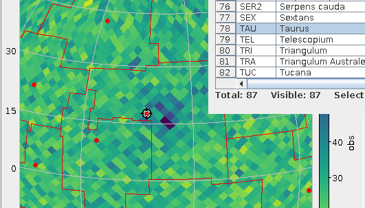
    GCNS density around taurus

    Taurus in the GCNS density plot: with constellations!

    So, since early March there's the cstl.geo table on the TAP service at https://dc.g-vo.org/tap with the constallation polygons in its p column. Which, for starters, means it's trivial to overplot constallation boundaries in your favourite VO clients now, as in the plot above. To make it, I've just done a boring SELECT * FROM cstl.geo, did the background (a plain HEALPix density plot of GCNS) and, clicked Layers → Add Area Control and selected the cstl.geo table.

    If you want to identify constellations by clicking, while in the area control, choose “add central” from the Forms menu in the Form tab; that's what I did in the figure above to ensure that what we're looking at here is the Hyades and hence Taurus. Admittedly: these “centres“ are – as in the catalogue – just the means of the vertices rather than the centres of mass of the polygon (which are hard to compute). Oh, and: there is also the AreaLabel in the Forms menu, for when you need the identification more than the table highlighting (be sure to use a center anchor here).

    Note that TOPCAT's polygon plot at this point is not really geared towards large polygons (which the constellations are) right now. At the time of writing, the documentation has: “Areas specified in this way are generally intended for displaying relatively small shapes such as instrument footprints. Larger areas may also be specified, but there may be issues with use.” That you'll see at the edges of the sky plots – but keeping that in mind I'd say this is a fun and potentially very useful feature.

    What's a bit worse: You cannot turn the constellation polygons into MOCs yet, because the MOC library currently running within our database will not touch non-convex polygons. We're working on getting that fixed.

    Nearby Stars

    Similarly tangible in my book is the GCNS: nearby stars I always find romantic.

    Let's look at the 100 nearest stars, and let's add spectral types from Henry Draper (cf. my post on Annie Cannon's catalogue) as well as the constellation name:

    WITH nearest AS (
    SELECT TOP 100
      a.source_id,
      a.ra, a.dec,
      phot_g_mean_mag,
      dist_50,
      spectral
    FROM gcns.main AS a
    LEFT OUTER JOIN hdgaia.main AS b
      ON (b.source_id_dr3=a.source_id)
    ORDER BY dist_50 ASC)
    SELECT nearest.*, name
    FROM nearest
    JOIN cstl.geo AS g
      ON (1=CONTAINS(
        POINT(nearest.ra, nearest.dec),
        p))
    

    Note how I'm using CONTAINS with the polygon in the constellations table here; that's the usage I've had in mind for this table (and it's particularly handy with table uploads).

    That I have a Common Table Expression (“WITH”) here is due to SQL planner confusion (I'll post something about that real soon now): With the WITH, the machine first selects the nearest 100 rows and then does the (relatively costly) spatial match, without it, the machine (somewhat surprisingly) did the geometric match first. This particular confusion looks fixable, but for now I'd ask you for forgiveness for the hack – and the technique is often useful anyway.

    If you inspect the result, you will notice that Proxima Cen is right there, but α Cen is missing; without having properly investigated matters, I'd say it's just too bright for the current Gaia data reduction (and quite possibly even for future Gaia analysis).

    Most of the objects on that list that have made it into the HD (i.e., have a spectral type here) are K dwarfs – which is an interesting conspiracy between the limits of the HD (the late red and old white dwarfs are too weak for it) and the limits of Gaia (the few earlier stars within 6 parsec – which includes such luminaries as Sirius at a bit more than 2.5 pc – are just too bright for where Gaia data reduction is now).

    Animation

    Another fairly tangible thing in the GCNS is the space velcity, given in km/s in the three dimensions U, V, and W. That is, of course, an invitation to look for stellar streams, as, within the relatively small portion of the Milky Way the GCNS looks at, stars on similar orbits will exhibit similar space motions.

    Considering the velocity dispersion within a stellar stream will be a few km/s, let's have the database bin the data. Even though this data is small enough to conveniently handle locally, this kind of remote analysis is half of what TAP is really great at (the other half being the ability to just jump right into a new dataset). You can group by multiple things at the same time:

    SELECT
      COUNT(*) AS n,
      ROUND(uvel_50/5)*5 AS ubin,
      ROUND(vvel_50/5)*5 AS vbin,
      ROUND(wvel_50/5)*5 AS wbin
    FROM gcns.main
    GROUP BY ubin, vbin, wbin
    

    Note that this (truly) 3D histogram only represents a small minority of the GCNS objects – you need radial velocities for space motion, and these are precious even in the Gaia age.

    What really surprised me is how clumpy this distribution is – are we sure we already know all stellar streams in the solar neighbourhood? Watch for yourself (if your browser can't play webm, complain to your vendor):

    [Update (2021-04-01): Mark Taylor points out that the “flashes” you sometimes see when the grid is aligned with the viewing axes (and the general appearance) could be improved by just pulling all non-NULL UVW values out of the table and using a density plot (perhaps shading=density densemap=inferno densefunc=linear). That is quite certainly true, but it would of course defeat the purpose of having on-server aggregation. Which, again, isn't all that critical for this dataset, so doing the prettier plot actually is a valuable exercise for the reader]

    How did I make this video? Well, I started with a Cube Plot in TOPCAT as usual, configuring weighted plotting with n as its weight and played around a bit with scaling out a few outliers. And then I saved the table (to zw.vot), hit “STILTS“ in the plot window and saved the text from there to a text file, zw.sh. I had to change the ``in`` clause in the script to make it look like this:

    #!/bin/sh
    stilts plot2cube \
     xpix=887 ypix=431 \
     xlabel='ubin / km/s' ylabel='vbin / km/s' \
     zlabel='wbin / km/s' \
     xmin=-184.5 xmax=49.5 ymin=-77.6 ymax=57.6 \
     zmin=-119.1 zmax=94.1 phi=-84.27 theta=90.35 \
      psi=-62.21 \
     auxmin=1 auxmax=53.6 \
     auxvisible=true auxlabel=n \
     legend=true \
     layer=Mark \
        in=zw.vot \
        x=ubin y=vbin z=wbin weight=n \
        shading=weighted size=2 color=blue
    

    – and presto, sh zw.sh would produce the plot I just had in TOPCAT. This makes a difference because now I can animate this.

    In his documentation, Mark already has a few hints on how to build animations; here are a few more ideas on how to organise this. For instance, if, as I want here, you want to animate more than one variable, stilts tloop may become a bit unwieldy. Here's how to give the camera angles in python:

    import sys
    from astropy import table
    import numpy
    
    angles = numpy.array(
      [float(a) for a in range(0, 360)])
    table.Table([
        angles,
        40+30*numpy.cos((angles+57)*numpy.pi/180)],
      names=("psi", "theta")).write(
        sys.stdout, format="votable")
    

    – the only thing to watch out for is that the names match the names of the arguments in stilts that you want to animate (and yes, the creation of angles will make numpy afficionados shudder – but I wasn't sure if I might want to have somewhat more complex logic there).

    [Update (2021-04-01): Mark Taylor points out that all that Python could simply be replaced with a straightforward piece of stilts using the new loop table scheme in stilts, where you would simply put:

    animate=:loop:0,360,0.5
    acmd='addcol phi $1'
    acmd='addcol theta 40+30*cosDeg($1+57)'
    

    into the plot2cube command line – and you wouldn't even need the shell pipeline.]

    What's left to do is basically the shell script that TOPCAT wrote for me above. In the script below I'm using a little convenience hack to let me quickly switch between screen output and file output: I'm defining a shell variable OUTPUT, and when I un-comment the second OUTPUT, stilts renders to the screen. The other changes versus what TOPCAT gave me are de-dented (and I've deleted the theta and psi parameters from the command line, as I'm now filling them from the little python script):

    OUTPUT="omode=out out=pre-movie.png"
    #OUTPUT=omode=swing
    
    python3 camera.py |\
    stilts plot2cube \
       xpix=500 ypix=500 \
       xlabel='ubin / km/s' ylabel='vbin / km/s' \
       zlabel='wbin / km/s' \
       xmin=-184.5 xmax=49.5 ymin=-77.6 ymax=57.6 \
       zmin=-119.1 zmax=94.1 \
       auxmin=1 auxmax=53.6 \
    phi=8 \
    animate=- \
    afmt=votable \
    $OUTPUT \
       layer=Mark \
          in=zw.vot \
          x=ubin y=vbin z=wbin weight=n \
          shading=weighted size=4 color=blue
    
    # render to movie with something like
    # ffmpeg -i "pre-movie-%03d.png" -framerate 15 -pix_fmt yuv420p /stream-movie.webm
    # (the yuv420p incantation is so real-world
    # web browsers properly will not go psychedelic
    # with the colours)
    

    The comment at the end says how to make a proper movie out of the PNGs this produces, using ffmpeg (packaged with every self-respecting distribution these days) and yielding a webm. Yes, going for mpeg x264 might be a lot faster for you as it's a lot more likely to have hardware support, but everything around mpeg is so patent-infested that for the sake of your first-born's soul you probably should steer clear of it.

    Movies are fun in webm, too.

  • Automating TAP queries

    TOPCAT is a great tool – in particular, for prototyping and ad-hoc analyses, it's hard to beat. But say you've come up with this great TAP query, and you want to preserve it, perhaps generate plots, then maybe fix them when you (or referees) have spotted problems.

    Then it's time to get acquainted with TOPCAT's command line sister STILTS. This tool lets you do most of what TOPCAT can, but without user intervention. Since the command lines usually take a bit of twiddling I usually wrap stilts calls with GNU make, so I just need to run something like make fig3.pdf or make fig3.png and make figures out what to do, potentially starting with a query. Call it workflow preservation if you want.

    How does it work? Well, of course with a makefile. In that, you'll first want to define some variables that allow more concise rules later. Here's how I usually start one:

    STILTS?=stilts
    
    # VOTables are the results of remote queries, so don't wantonly throw
    # them away
    .PRECIOUS: %.vot
    
    # in this particular application, it helps to have this global
    HEALPIX_ORDER=6
    
    # A macro that contains common stuff for stilts TAP query -- essentially,
    # just add adql=
    TAPQUERY=$(STILTS) tapquery \
      tapurl='http://dc.g-vo.org/tap' \
      maxrec=200000000 \
      omode=out \
      out=$@ \
      ofmt=vot \
      executionduration=14400
    
    # A sample plot macro.  Here, we do a healpix plot of some order. Also
    # add value_1=<column to plot>
    HEALPIXPLOT=$(STILTS) plot2sky \
      auxmap=inferno \
      auxlabel='$*'\
      auxvisible=true \
      legend=false \
      omode=out \
      out=$@ \
      projection=aitoff \
      sex=false \
      layer_1=healpix \
        datalevel_1=$(HEALPIX_ORDER) \
        datasys_1=equatorial \
        viewsys_1=equatorial \
        degrade_1=0 \
        transparency_1=0 \
        healpix_1=hpx \
        in_1=$< \
        ifmt_1=votable \
        istream_1=true \
    

    For the somewhat scary STILS command lines, see the STILTS documentation or just use your intution (which mostly should give you the right idea what something is for).

    The next step is to define some pattern rules; these are a (in the syntax here, GNU) make feature that let you say „to make a file matching the destination pattern when you have one with the source pattern, use the following commands”. You can use a number of variables in the rules, in particular $@ (the current target) and $< (the first prerequisite). These are already used in the definitions of TAPQUERY and HEALPIXPLOT above, so they don't necessarily turn up here:

    # healpix plots from VOTables; these will plot obs
    %.png: %.vot
          $(HEALPIXPLOT) \
                  value_1=obs \
                  ofmt=png \
                  xpix=600 ypix=380
    
     %.pdf: %.vot
           $(HEALPIXPLOT) \
                   value_1=obs \
                   ofmt=pdf
    
     # turn SQL statements into VOTables using TAP
     %.vot: %.sql
           $(TAPQUERY) \
                  adql="`cat $<`"
    

    Careful with cut and paste: The leading whitespace here must be a Tab in rules, not just some blanks (this is probably the single most annoying feature of make. You'll get used to it.)

    What can you do with it? Well, for instance you can write an ADQL query into a file density.sql; say:

    SELECT
      count(*) as obs,
      -- "6" in the next line must match HEALPIX_ORDER in the Makefile
      ivo_healpix_index (6, alphaFloat, deltaFloat) AS hpx
    FROM ppmx.data
    GROUP BY hpx
    

    And with this, you can say:

    make density.pdf
    

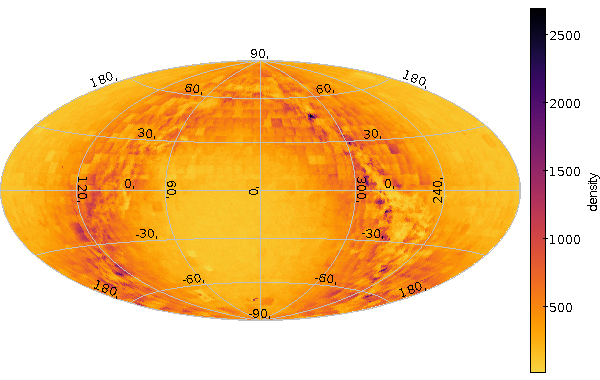
    and get a nice PDF with the plot resulting from that query. Had you just said make density.vot, make would just have executed the query and left the VOTable, e.g., for investigation with TOPCAT, and if you were to type make density.png, you'd get a nice PNG without querying the service again. Like this:

    A density plot

    Unless of course you changed the SQL in the meantime, in which case make would figure out it had to go back to the service.

    In particular for the plots you'll often have to override the defaults. Make is smart enough to figure this out. For instance, you could have two files like this:

    $ cat pm_histogram.sql
    SELECT
      round(pmtot/10)*10 as bin, count(*) as n
    FROM (
      SELECT sqrt(pmra*pmra+pmde*pmde)*3.6e6 as pmtot
      FROM hsoy.main) AS q
    group by bin
    $ cat pm_histogram_cleaned.vot
    SELECT
      round(pmtot/10)*10 as bin,
      count(*) as n
      FROM (
        SELECT sqrt(pmra*pmra+pmde*pmde)*3.6e6 as pmtot
        FROM hsoy.main
        WHERE no_sc IS NULL) AS q
      group by bin
    

    (these were used to analyse the overall proper motions distributions in HSOY properties; note that each of these will run about 30 minutes or so, so better adapt them to what's actually interesting to you before trying this).

    No special handling in terms of queries is necessary for these, but the plot needs to be hand-crafted:

    pm_histograms.png: pm_histogram.vot pm_histogram_cleaned.vot
         $(STILTS) plot2plane legend=false \
                 omode=out ofmt=png out=$@ \
                  title="All-sky" \
                  xpix=800 ypix=600 \
                  ylog=True xlog=True\
                  xlabel="PM bin [mas/yr, bin size=10]" \
                  xmax=4000 \
                  layer1=mark \
                         color1=blue \
                         in1=pm_histogram.vot \
                         x1=bin \
                         y1=n \
                 layer2=mark \
                         in2=pm_histogram_cleaned.vot \
                         x2=bin \
                         y2=n
    

    – that way, even if you go back to the stuff six months later, you can still figure out what you queried (the files are still there) and what you did then.

    A makefile to play with (and safe from cut-and-paste problems) is available from Makefile_tapsample (rename to Makefile to reproduce the examples).

Page 1 / 1