![[RSS]](../theme/image/rss.png)
Computing Residuals of an Astrometric Calibration
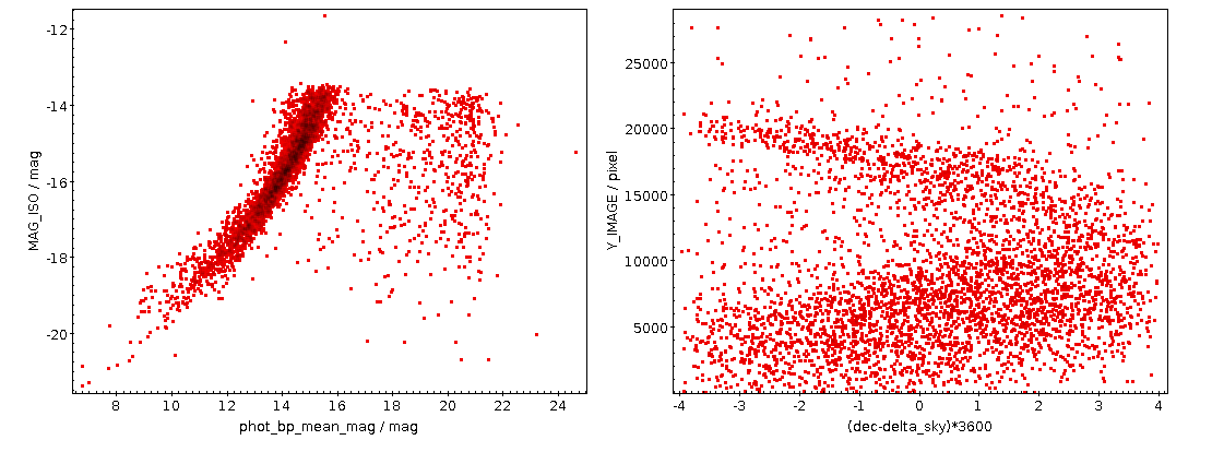
The kind of plot you can make following the recipe given here: Left, a comparison of the photometry, right, a positional residuals, not taking into account the SIP plate solution, when comparing the HDAP plate B3261a against Gaia DR3. Note that the cut-off a 4 arcsec is because of the match radius when obtaining the calibrator stars.
I recently had to assess the quality of the astrometric calibration of a photographic plate. What I am going to show you in this post will of course work just as well for CCD frames, and if these have a sufficiently large field of view, this may be an issue for them as well. However, the sort of data that needs this assessment most typically are scans of plates, as these tend to have a “wobble”, systematic offsets in the scan direction resulting from imperfections in the mechanics.
Prerequisites: An astronomical frame with a calibration in ICRS (or some frame not very far from it), called my-image.fits in the following, SExtractor (in Debian and derivatives: apt install source-extractor – long live Debian Astro; since it's called source-extractor in Debian, that's what I'll use here, too), and of course TOPCAT.
Step 1: Extract Sources. Source extraction is of course a high science, and if you know better than me, by all means do it the way you think is appropriate. Meanwhile, the following might very well work for you sufficiently well.
Create a working directory and enter it. Then, to create a file telling source-extractor what columns you would like to see, write the following to a file default.param:
ALPHA_SKY
DELTA_SKY
X_IMAGE
Y_IMAGE
MAG_ISO
FLUX_AUTO
ELONGATION
Next, give a few parameters to source-extractor; depending on the sort of image you have, you may want to play around with DETECT_MINAREA (how many pixels need to show a signal to register as a source) and DETECT_THRESH (how many sigmas a pixel has to be above the background to register as a candidate for belonging to a source). Meanwhile, write the following into a file default.control:
CATALOG_TYPE     FITS_1.0
CATALOG_NAME     img.axy
PARAMETERS_NAME  default.param
FILTER           N
DETECT_MINAREA   30
DETECT_THRESH    4
SEEING_FWHM      1.2
– but if the following call gives you a few hundred sources, that ought to work for the present purpose.
Then run:
source-extractor -c default.control my-image.fits
This will give you a catalogue of extracted objects in the file img.axy.
Step 2: Fix source-extractor's output. Load that img.axy into TOPCAT. Regrettably, source-extractor does not add any useful metadata to the columns of its output table. To add the absolute bare minimum, in TOPCAT go to Views → Column Info. In that window, check UCD in the Display menu, and then put pos.eq.ra and pos.eq.dec into the UCD fields of the ALPHA_SKY and DELTA_SKY columns, respectively; double click to change fields in TOPCAT.
To see if you have done the annotation right, in TOPCAT's main window, click Graphics → Sky Plot. If the objects show up, you have just provided enough annotation to let TOPCAT figure out the position for each row.
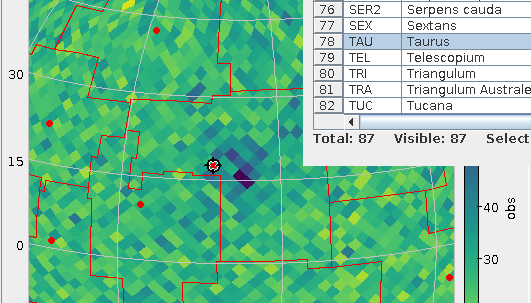
Step 3: Get calibrators. We will now try to add counterparts for Gaia DR3 to the extracted sources. To do that, click VO → Table Access Protocol, and in the window popping up double click the entry for the GAVO DC TAP.
In the Find box, type dr3lite to look for this site's version of the Gaia DR3 source catalogue. Click on gaia.dr3lite to select that table, and then select the Columns pane. This should show some of the Gaia DR3 columns.
Now Examples → Upload Join will generate a query that will cross-match your extracted sources with the Gaia sources. You should edit it a bit, only selecting the columns you will actually need, removing the TOP 1000 (at least on large images with more than 1000 sources), and reducing the match radius a bit when the calibration is not actually completely off and your epoch is sufficiently close to J2000.
Hint: you can control-click in the Columns pane and then use the Cols button to insert all the column names in one go[1]. For me, the resulting query would be:
SELECT
   source_id, ra, dec, phot_bp_mean_mag,
   tc.*
   FROM gaia.dr3lite AS db
   JOIN TAP_UPLOAD.t1 AS tc
   ON 1=CONTAINS(POINT('ICRS', db.ra, db.dec),
                 CIRCLE('ICRS', tc.ALPHA_SKY, tc.DELTA_SKY, 4./3600.))
This should result in about as many matches as your extraction had – a few more is ok, because you will have some spurious matches, a few less is ok, too, as there are always some outliers and artefacts, but you should clearly not pull a magnitude more or less objects here than you put in; fiddle with the match radius as necessary.
See if there is a rough correlation between the Gaia calibrators and your extracted sources by plotting phot_bp_mean_mag against MAG_ISO. Absent more information, MAG_ISO, source-extractor's guess for the magnitude of the extracted object, will be just some crazy number, but it should have some discernable correlation with the actual magnitude. Do not expect too much here, in particular with old plates, for which good photometry is a science of their own.
In my example, this looked like this:
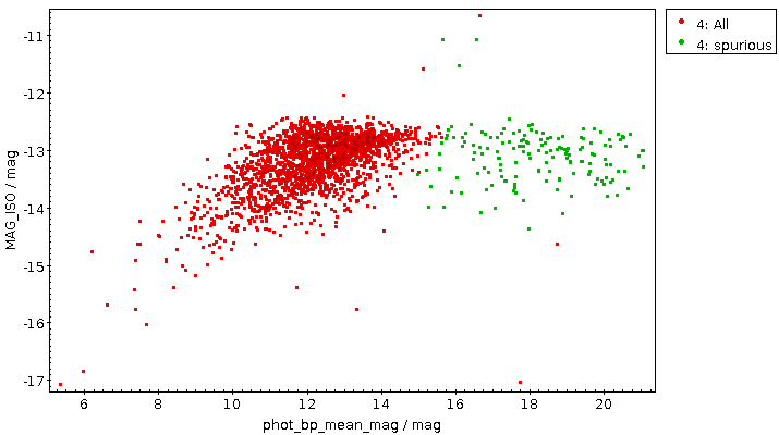
The green points certainly are spurious matches; this observation did not reach beyond 14th magnitude or so, and there are many weak stars on the sky, so a few of them will show up in just about any cross match. See the opening picture for an example with a better correlation.
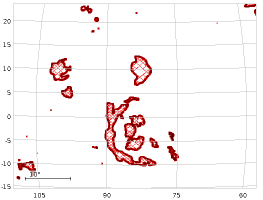
Step 4: Do the correlation plot. Do Graphics → Plane Plot and then plot ra-alpha_sky or dec-delta_sky against X_IMAGE or Y_IMAGE. You could get something like this:
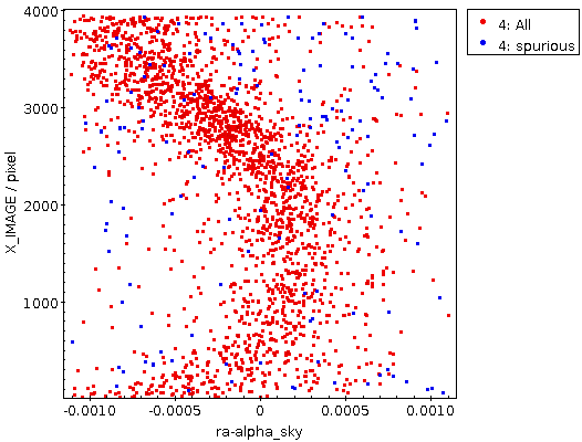
This rather certainly reflects some optical distortion; source-extractor regrettably does not take into account SIP corrections yet, so it is likely that a large part of this would be taken care of by the polynomials of the plate solution (the github issue I am linking to tells you how to be sure).
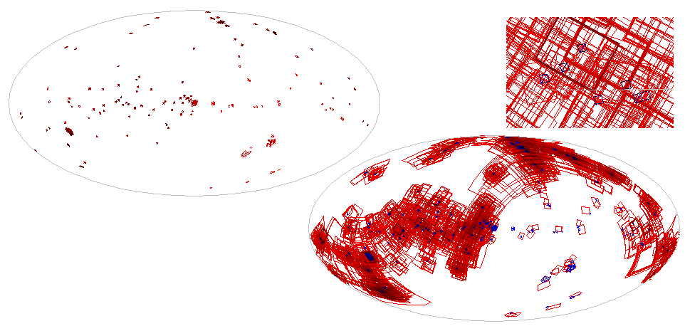
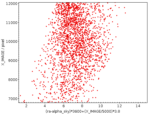
But it can also look like this:
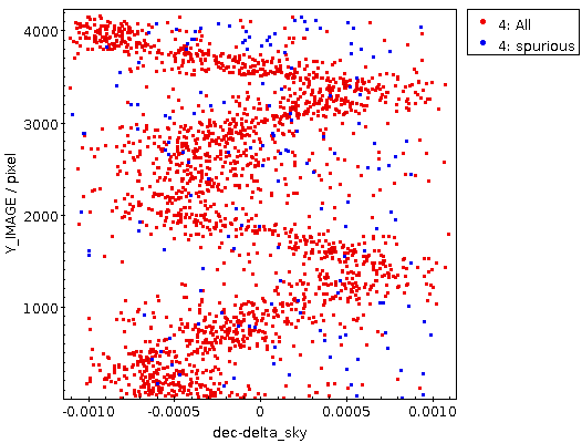
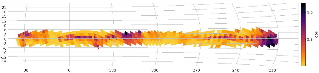
This certainly is not the result of a lens or anything optical at all. It's the scanner's gears that you are looking at here. With an amplitude of perhaps three arcseconds this is rather excessive here; but something like this you will rather likely see even on good scanners – though it may essentially be invisible, as of the Heidelberg scanner we used for HDAP:
| [1] | I'm using the BP magnitude in the query below as most historical plates tend to be “blue sensitive“ (in some sense). Hence, BP magnitudes should be a bit closer to what source-extractor has extracted. |