DaCHS 1.2 is out
Today, I have released DaCHS 1.2 – somewhat belatedly perhaps, because I managed to break my collarbone, but here it is. If you've been following this blog, you already know about the headline news: the dachs start command, ADQL 2.1, and early support for STC in the registry.
If you're not yet on DaCHS 1.1, please have a quick look at the corresponding release article. While the upgrade itself should work fine in one go even from older versions, the release notes of course apply cumulatively, and you may still have to do the dist-upgrade to 1.1.
As usual, the generic upgrading instructions are available in the operator's guide (in short: do a dachs val ALL; apt update; apt upgrade). Since I've still encountered DaCHS installations with wrong sources.lists last April: Note again that our repository names have changed in August 2016 – we now have release and beta rather than Debian release names. So, make sure you have something like:
deb http://vo.ari.uni-heidelberg.de/debian release main
in your /etc/apt/sources.list, not something containing “stable” or the like.
That said, here's the commented changes for 1.2:
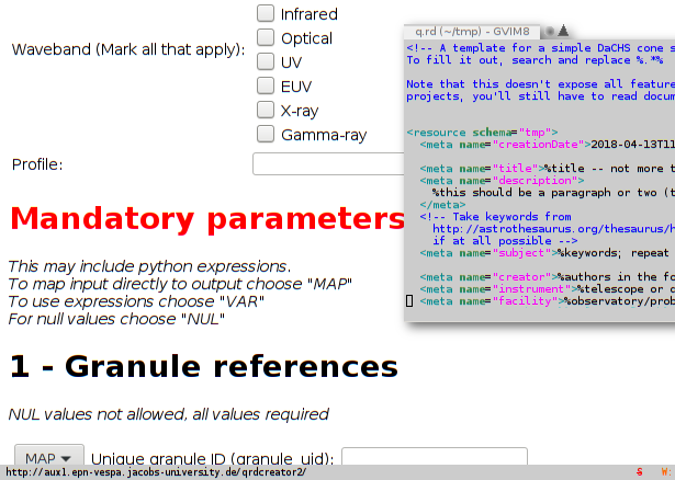
- New dachs start command to produce structured templates for certain service types. See Horror Vacui Begone on this blog for the full story.
- Support for ADQL 2.1 (actually, its current proposed recommendation), including almost all of the optional parts (see Speak out on ADQL 2.1 on this blog). While not strictly necessary, it's a good idea to run dachs imp //adql after the upgrade; this will give you some nice new UDFs, in particular gavo_histogram.
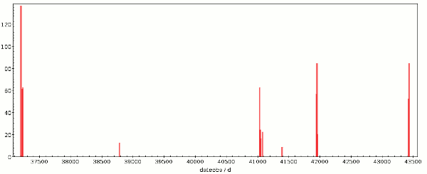
- New coverage element (with updaters) to build and declare the space-time-spectral coverage of a resource. It would be great if you could add coverage elements to your resources where it makes sense and re-publish them. This blog post tells you how to do it (you'll have to scroll down a bit).
- There is now odbcGrammar to feed an import from another database. Essentially, you put an ODBC connection string into a file, point your sources element there, and you'll get one rawdict per tuple in a foreign database table. This might be a nice way to publish moderate-size non-postgres tables via DaCHS.
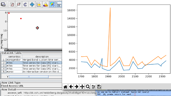
- You can now declare associated datalink services for tables using the _associatedDatalinkSvc meta item. In particular, if you had a datalink property on SSAP services, you should migrate at some point. One advantage: Users will get the datalinks even when querying the tables through TAP. See “Integrating Datalink Services” in the reference documentation for the full story.
- We now force matplotlib to read its configuration from /var/gavo/etc/matplotlibrc; to get a default, just run dachs init again. This is mainly to avoid uncontrolled imports of matplotlibrcs when DaCHS is run under a uid that does other things now and then.
- DaCHS now supports VOSI 1.1; in particular, DaCHS now understands the detail hints and has per-table endpoints, so clients like TOPCAT could avoid reading the full table metadata in one go. Realistically, at least TOPCAT doesn't yet, so this is perhaps less cool than it may sound.
- The indices generated by the ssa mixins are now a bit more sensible considering typical query modes. You probably want to run dachs imp -I on the RDs for your ssap data collections when convenient. If you have larger spectral collections, chances are many queries will be a lot faster.
- ssapCore no longer wantonly adds preview columns. If you have previews with spectra, you probably want to add <property name="previews">auto</property> to your ssapCores. If you don't, the preview column will not be added to SSA responses (right now, few clients evaluate it, but that will hopefully change in the future).
- You can now add a statisticsTarget property to columns; you will want this on largish tables with non-uniformly distributed values to aid the query planner; something like <property key=" statisticsTarget">10000</property> within the corresponding column element can go a long way to improve query planning (you need to run gavo imp -m on the RD after the change).
- DaCHS's log now by default does not contain IP addresses, user agents, and referrers any more, which should mostly keep you from processing personal data and thus from having to muck around with the EU GDPR. To get back the previous behaviour, set [web]logFormat in /etc/gavo.rc to combined.
- I fixed some utypes for obscore 1.1. These utypes are useless, so there's nothing you have to do. But then stilts taplint complains about them, and so you may want to run dachs imp -m //obscore.
- As usual, there are many minor bug fixes and improvements (e.g., memmapping FITSes for cutout again, delimited table references in ADQL, new-style tutorial resource records, correct obscore standardId, much saner nD-arrays in VOTables).
Well – enjoy the release, and if something goes wrong with it, be sure to let us know, preferably on the DaCHS-suppport mailing list.

![[RSS]](./theme/image/rss.png)


