![[RSS]](./theme/image/rss.png)
LAMOST5 meets Datalink
One of the busiest spectral survey instruments operated right now is the Large Sky Area Multi-Object Fiber Spectrograph Telescope (LAMOST). And its data in the VO, more or less: DR2 and DR3 have been brought into the VO by our Czech colleagues, but since they currently lack resources to update their services to the latest releases, they have kindly given me their DaCHS resource descriptor, and so I had a head start for publishing DR5 in Heidelberg.
With some minor updates, here it is now: Over nine million medium-resolution spectra covering large parts of the northen sky – the spatial coverage is like this:
There's lots of fun to be had with this; of course, there's an SSA service, so when you point Aladin or Splat at some part of the covered sky and look for spectra, chances are you'll see LAMOST spectra, and when working on some of our tutorials (this one, for example), it happened that LAMOST actually had what I was looking for when writing them.
But I'd like to use the opportunity to mention two other modes of accessing the data.
Tablesample and TOPCAT's Plot Table activation action
Say you'd like to look at spectra of M stars and would like to have some sample from across the sky, fire up TOPCAT, point its TAP client the GAVO DC TAP service (http://dc.g-vo.org/tap) and run something like:
select
  ssa_pubDID, accref, raj2000, dej2000, ssa_targsubclass
from lamost5.data tablesample(1)
where
  ssa_targsubclass like 'M%'
This is using the TABLESAMPLE modifier in the from clause, which isn't standard ADQL yet. As mentioned in the DaCHS 1.4 announcement, DaCHS has a prototype implementation of what's been discussed on the IVOA's DAL mailing list: pick a part of a table rather than the full one. It takes a percentage as an argument, and tells the server to choose about this percentage of the table's records using a reasonable and fast heuristic. Note that this won't give you perfect statistical sampling, but if it's not “good enough” for some purpose, I'd like to learn about that purpose.
Drawing a proper statistical sample, on the other hand, would take minutes on the GAVO database server – with tablesample, I had the roughly 6000 spectra the above query returns essentially instantaneously, and from eyeballing a sky plot of them, I'd say their distribution is close enough to that of the full DR5. So: tablesample is your friend.
For a quick look at the spectra themselves, in TOPCAT click Views/Activation Actions, check “Plot Table” and make sure TOPCAT proposes the accref column as “Table Location” (if you don't see these items, update your TOPCAT – it's worth it). Now click on a row or perhaps a dot on a plot and behold an M spectrum.
Cutouts via Datalink
LAMOST releases spectra in FITS format pretty much like the ones you may know from SDSS. The trick above works because we instead hand out proper, IVOA Spectral Data Model-compliant spectra through SSA and TAP. However, if you need to go back to the original files, you can, using Datalink. If you're unsure what this Datalink thing is: call me vain, but I still like my 2015 ADASS poster explaining that. In TOPCAT, you'd be using the “Invoke Service” activation action to get to the datalinks.
If you have actual work to do, offloading repetetive work to the computer is what you want, and fortunately, pyVO knows about datalink, too. I give you this is hard to discover so far, and the interface is... a tiny bit clunky. Until some kind soul cleans up the pyVO datalink act, a poster Stefan and I showed at the 2017 ADASS might give you an idea which buttons to press. Or read on and see how things work for LAMOST5.
The shortest way to datalinks is a TAP query that at least retrieves the ssa_pubdid column (that's a must; Datalink can't work without it) and, on the result, run the iter_datalinks method. This returns an object in which you can find the associated data items (in this case, a preview and the original FITS with the #progenitor semantics), plus the cutout service.
Hence, a minimal example for pulling the legacy FITS links out of the first three items in lamost5.data would look like this:
import pyvo

svc = pyvo.dal.TAPService("http://dc.g-vo.org/tap")
for dl in svc.run_sync("select top 3 ssa_pubdid"
        " from lamost5.data").iter_datalinks():
    print(next(dl.bysemantics("#progenitor")
        )["access_url"].decode("ascii"))
This is a bit different from listing 2 in the poster linked above because it's python3, so getting the first element from iterator an iterator looks a bit different, and (curse astropy.votable for returning VOTable chars as bytes rather than strings!) you'll want to turn the URL into a proper string manually.
Another, actually more interesting, thing you can do with Datalink is cut out regions of interest. The LAMOST spectra are fairly long (though of course still small by image standards), so if you're only interested in a single line, you can save a bit of storage and bandwidth over blindly pulling the whole thing.
For instance, if you wanted to pull the vicinity of the H and K Fraunhofer lines from the matches in the loop in the snippet above, you could say:
from astropy import units as u
proc = next(dl.iter_procs())
cutout = proc.processed(band=(392*u.nm,398*u.nm))
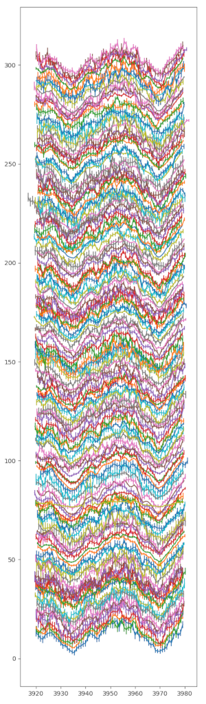
And this is what I've done for the decorative left border above: it's the H and K line profiles for 0.1% of the stars LAMOST has classified as G8. Building the image didn't take more than a few seconds (where I'd like the cutouts to be faster by a factor of 10; I guess that's about an afternoon of work for me, so if it'd save you more than that afternoon, poke me to do it).
What's coming back is tables. By the time python has digested these, they're numpy record arrays. Thus, you can immediately bring in your beloved scipy (or whatever). For instance, if for some reason you're convinced that the H and K lines should be fit by identical Gaussians in the boring case and would like find objects for which that's patently untrue and that hence could be un-boring, here's how you could do that:
def spectral_model(wl, c1, c2, depth, width):
    return (1
        -depth*numpy.exp(-numpy.square(wl-c1)
            /numpy.square(width))
        -depth*numpy.exp(-numpy.square(wl-c2)
            /numpy.square(width)))

for pubdid, prof in get_profiles(
        "G8", (392*u.nm,398*u.nm), 0.01, 4):
    prof["flux"] /= max(prof["flux"])
    popt, pcov = curve_fit(
        spectral_model, prof["spectral"], prof["flux"],
        sigma=prof["flux_error"],
        p0=[3968, 3934, 1, 1])
    if pcov[3][3]>1:
        break
– where get_profiles is essentially doing the TAP plus datalink routine above, except I'm swallowing spectra with too much noise and I have the function transform the spectral coordinate into the objects' rest frames. If you're curious how I'm doing this just based on the IVOA Spectral Data Model, check the source linked at the bottom of this post.
I've just run this, and the first spectrum that the machinery flagged as suspicious was this:
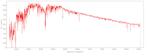
– which doesn't look like I've made a discovery just yet. But that doesn't mean there's not a lot to find within LAMOST5's lines...
To get you up to speed quickly: here's the actual python3 code I ran for the “analysis” and the plot.