2024-11-14
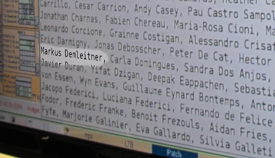
Markus Demleitner
It is Interop time again! Most people working on the Virtual
Observatory are convened in Malta at the moment and will discuss the
development and reality of our standards for the next two days. As
usual, I will report here on my thoughts and the proceedings
as I go along, even though it
will be a fairly short meeting: In northen autumn, the Interop always is
back-to-back with ADASS, which means that most participants already have
3½ days of intense meetings behind them and will probably be particularly
glad when we will conclude the Interop Sunday noon.
The TCG discusses (Thursday, 15:00)
Right now, I am sitting in a session of the Technical
Coordination Group, where the chairs and vice-chairs of the Working
and Interest Groups meet and map out where they want to go and how it
all will fit together. If you look at this meeting's agenda, you can
probably guess that this is a roller coaster of tech and paperwork,
quickly changing from extremely boring to extremely exciting.
For me up to now, the discussion about whether or not we want LineTAP
at all was the most relevant agenda item;
while I do think VAMDC would win by taking
up the modern IVOA TAP and Registry standards (VAMDC was forked from the VO
in the late 2000s), takeup has been meagre so far, and so perhaps this
is solving a problem that nobody feels.
I have frankly (almost) only
started LineTAP to avoid a SLAP2 with an accompanying data model that
would then compete with XSAMS, the data model below VAMDC.
On the other hand: I think LineTAP works so much more nicely than VAMDC
for its use case (identify spectral lines in a plot) that it would
be a pity to simply bury it.
By the way, if you want, you can follow the (public; the TCG meeting is
closed) proceedings online; zoom links are available from the programme
page. There will be recordings later.
At the Exec Session (Thurday, 16:45)
The IVOA's Exec is where the heads of the national projects meet,
with the most noble task of endorsing our recommendations and otherwise
providing a certain amount of governance. The agenda of Exec
meetings is public, and so will the minutes be, but otherwise this again is a
closed meeting so everyone feels comfortable speaking out. I certainly
will not spill any secrets in this post, but rest assured that there are
not many of those to begin with.
That I am in here is because GAVO's actual head, Joachim, is not on Malta and
could not make it for video participation, either. But then someone from GAVO
ought to be here, if only because a year down the road, we
will host the Interop: In the northern autumn of 2025, the ADASS and the
Interop will take place in Görlitz (regular readers of this blog have
heard of that town before), and so I see part of my role in this
session in reconfirming that we are on it.
Meanwhile, the next Interop – and determining places is also the Exec's
job – will be in the beginning of June 2025 in College Park, Maryland.
So much for avoiding flight shame for me (which I could for Malta that
still is reachable by train and ferry, if not very easily).
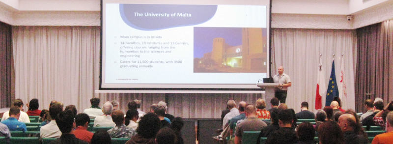
Opening Plenary (Friday 9:30)
Interops always begin with a plenary with reports from the various
functions: The chair of the Exec, the chair of the committee of science
priorities, and chair of technical coordination group. Most
importantly, though, the chairs of the working and interest groups
report on what has happened in their groups in the past semester, and
what they are planning for the Interop (“Charge to the working
groups”).
For me personally, the kind words during Simon's State of the IVOA
report on my VO lecture (parts of which he has actually reused) were
particularly welcome.
But of course there was other good news in that talk. With my Registry
grandmaster hat on, I was happy to learn that NOIRLabs has
released a simple publishing registry implementation, and
that ASVO's (i.e., Australia) large TAP server will finally be properly registered, too.
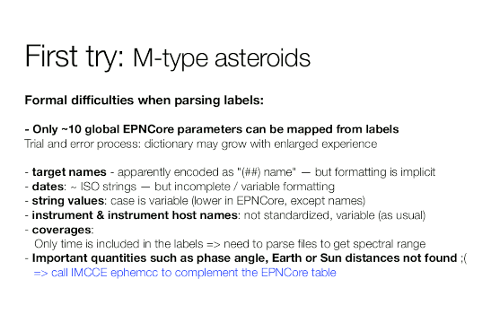
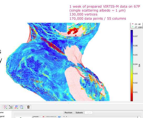
The prize for the coolest image, though, goes to VO France and in
particular their solar system folks, who have used TOPCAT to visualise
data on a model of comet 67P Churyumov–Gerasimenko (PDF page 20).
Self-Agency (Friday, 10:10)
I have to admit it's kind of silly to pick out this particular point
from all the material discussed by the IG and WG chairs in the Charge
to the Working Groups, but a part of why this job is so gratifying is
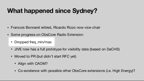
experiences of self-agency. I just had one of these during the Radio
IG report: They have dropped the duplication of spectral information
in their proposed extension to obscore.
Yay! I have lobbied for that
one for a long time on grounds that if there is both em_min/em_max
and f_min/f_max in an obscore records (which express the same thing,
with em_X being wavelengths in metres, and f_X frequencies in… something
else, where proposals included Hz, MHz and GHz),
it is virtually certain that at least one pair is wrong. Most
likely, both of them will be. I have actually created a UDF for ADQL
queries to make that point. And now: Success!
Focus Session: High Energy and Time Domain (Friday, 12:00)
The first “working” session of the Interop is a plenary on High Energy
and Time Domain, that is, instruments that look for messenger
particles that may have the energy of a tennis ball, as well as ways to let
everyone else know about them quickly.
Incidentally, that “quickly” is a reason for why the
two apparently unconnected topics share a session: Particles
in the tennis ball range
are fortunately rare (or our DNA would be in trouble), and so when you
have found one, you might want make sure everone else gets to
look whether something odd shows up where that particle came from in
other messengers (as in: optical photons, say). This is also relevant
because many detectors in that energy (and particle) range do not have a
particularly good idea of where the signal came from, and followups in
other wavelengths may help figuring out what sort of thing may have
produced a signal.
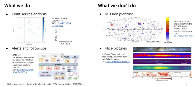
I enjoyed a slide by Jutta, who reported on VO publication of km3net
data, that is, neutrinos detected in a large detector cube below the
Mediterrenean sea, using the Earth as a filter:
“We don't do pretty pictures“ is of course a very cool thing one can
say, although I bet this is not 120% honest. But I am willing to give
Jutta quite a bit of slack; after all, km3net data is served through
DaCHS, and I am still hopeful that we will use it to prototype serving
more complex data products than just plain event lists in the future.
A bit later in the session, an excellent question was raised by Judy
Racusin in her talk on GCN:
The background of the question is that there is a rather reasonable
standard for the dissemination of alerts and similar data, VOEvent.
This has seen quite a bit of takeup in the 2000s, but, as evinced by
page 17 of Judy's slides, all the current large time-domain projects
decided to invent something new, and it seems each one invented
something different.
I don't have an definitive answer to why and how
that happened (as opposed to, for instance, everyone cooperating on
evolving VOEvent to match whatever requirements these projects have),
although outside pressures (e.g., the rise of Apache Avro and Kafka)
certainly played a role.
I will, however, say that I strongly suspect that if the VOEvent
community back then had had more public and registered streams consumed
by standard software, it would have been a lot harder for these new
projects to (essentially) ignore it. I'd suggest as a lesson to learn
from that: make sure your infrastructure is public and widely consumed
as early as you can. That ought to help a lot in ensuring that your
standard(s) will live long and prosper.
In Apps I (Friday 16:30)
I am now in the Apps session. This is the most show-and-telly
event you
will get at an Interop, with largest likelihood of encountering the
pretty pictures that Jutta had flamboyantly expressed disinterest in this morning.
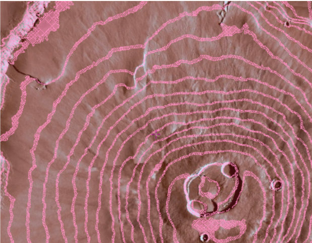
In the first talk already, Thomas delivers with, for
instance, mystic pictures from Mars:
Most of the magic was shown in a live demo; once the recordings are
online, consider checking this one out (I'll mention in passing that
HiPS2MOC looks like a very useful feature, too).
My talk, in contrast, had extremely boring slides; you're not missing
out at all by simply reading the notes. The message is not overly
nice, either: Rather do fewer features than optional ones, as a server
operator please take up new standards as quickly as you can, and in the
same role please provide good metadata. This last point happened to be
a central message in Henrik's talk on ESASky (which aptly followed mine)
as well, that, like Thomas', featured a live performance of eye candy.
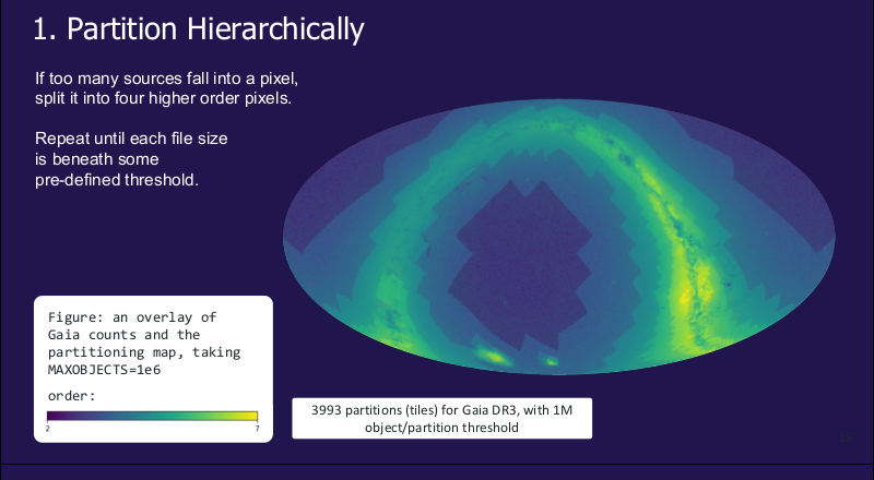
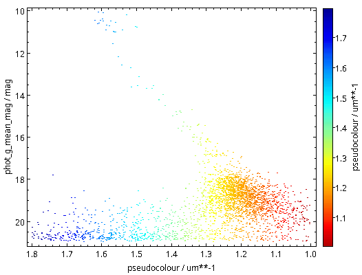
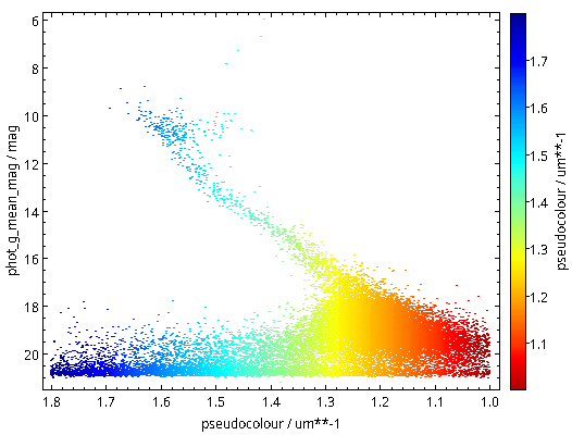
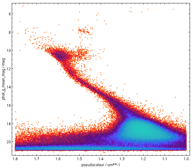
Mario Juric's talk on something called HATS then featured this nice
plot:
That's Gaia's source catalogue pixelated such that the sources in each
pixel require about a constant processing time. The underlying
idea, hierarchical tiling, is great and has proved itself extremely
capable not only with HiPS, which is what is behind basically anything
in the VO that lets you smoothly zoom, in particular Aladin's maps.
HATS' basic premise seems to be to put tables (rather than JPEGs or FITS
images as usual) into a HiPS structure. That has been done before, as
with the catalogue HiPSes; Aladin users will remember the Gaia or Simbad
layers. HATS, now, stores Parquet files, provides Pandas-like
interfaces on top of them, and in particular has the nice property of
handing out data chunks of roughly equal size.
That is certainly great, in particular for the humongous data sets that
Rubin (née LSST) will produce. But I wondered how well it will stand up
when you want to combine different data collections of this sort. The
good news: they have already tried it, and they even have thought about
how pack HATS' API behind a TAP/ADQL interface. Excellent!
Further great news in Brigitta's talk [warning: link to google]: It
seems you can now store ipython (“Jupyter”) notebooks in, ah well,
Markdown – at least in something that seems version-controllable. Note
to self: look at that.
Data Access Layer (Saturday 9:30)
I am now sitting in the first session of the Data Access Layer Working
Group. This is where we talk about the evolution of the protocols you
will use if you “use the VO”: TAP, SIAP, and their ilk.
Right at the start, Anastasia Laity spoke about a topic that has
given me quite a bit of headache several times already: How do you tell
simulated data from actual observations when you have just discovered a
resource that looks relevant to your research?
There is prior art for that in that SSAP has a data source metadata
item on complete services, with values survey, pointed, custom,
theory, or artificial (see also SimpleDALRegExt sect. 3.3, where
the operational part of this is specified). But that's SSAP only.
Should we have a place for that in registry records in general? Or even
at the dataset level? This seems rather related to the recent addition
of productTypeServed in the brand-new VODataService 1.3. Perhaps
it's time for dataSource element in VODataService?
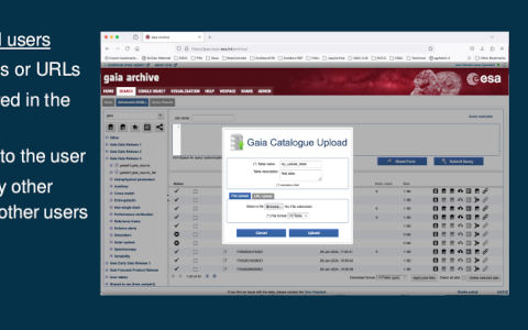
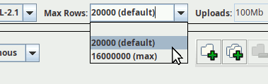
A large part of the session was taken up by the question of persistent
TAP uploads that I have covered here recently. I have summarised
this in the session, and after that, people from ESAC (who have built
their machinery on top of VOSpace) and CADC (who have inspired my
implementation) gave their takes on the topic of persistent uploads.
I'm trying hard to like ESAC's solution, because it is using the obvious
VO standard for users to manage server-side resources (even though the
screenshot in the slides,
suggests it's just a web page). But then it is an order of magnitude
more complex in implementation than my proposal, and the main advantage
would be that people can share their tables with other users. Is that a
use case important enough to justify that significant effort?
Then Pat's talk on CADC's perspective presented a hierarchy of use
cases, which perhaps offers a way to reconcile most of the opinions:
Is there is a point for having the same API on /tables and
/user_tables, depending on whether we want the tables to be publicly
visible?
Data Curation and Preservation (Saturday, 11:15)
This Interest Group's name sounds like something only a librarian could
become agitated about: Data curation and preservation. Yawn.
Fortunately, I am considering myself a librarian at heart, and hence I
am participating in the DCP session now. In terms of engagement, we
have already started to quarrel about a topic that must seem rather like
bikeshedding from the outside: should we bake in the DOI resolver into
the way we write DOIs (like
http://doi.org/10.21938/puTViqDkMGcQZu8LSDZ5Sg; actually, since a few
years: https instead of http?) or should we continue to use the doi URI
scheme, as we do now: doi:10.21938/puTViqDkMGcQZu8LSDZ5Sg?
This discussion came up because the doi foundation asks you to render
DOIs in an actionable way, which some people understand as them asking
people
to write DOIs with their resolver baked in. Now, I am somewhat reluctant to
do that mainly on grounds of user freedom. Sure, as long as you
consider the whole identifier an opaque string, their resolver is not
actually implied, but that's largely ficticious, as evinced by the fact
that somehow identifiers with http and with https would generally be
considered equivalent. I do claim that we should make it clear that
alternative resolvers are totally an option. Including ours: RegTAP
lets you resolve DOIs to ivoids and VOResource metadata, which to me
sounds like something you might absolutely want to do.
Another (similarly biased) point: Not
everything on the internet is http. There are other identifier types
that are resolvable (including ivoids).
Fortunately, writing DOIs as HTTP URIs is not actually what the doi
foundation is asking you to do. Thanks to Gus for clarifying
that.
These kinds of questions also turned up in the discussion after my talk
on BibVO. Among other things, that draft standard proposes to deliver
information on what datasets a paper used or produced in a very simple
JSON format. That parsimony has been put into question, and in the
end the question is: do we want to make our protocols a bit more
complicated to enable interoperability with other “things”, probably
from outside of astronomy? Me, I'm not sure in this case: I consider
all of BibVO some sort of contract essentially between the IVOA and SciX
(née ADS), and I doubt that someone else than SciX will even want
to read this or has use for it.
But then I (and others) have been wrong with preditions like this before.
Registry (Saturday 14:30)
Now it's registry time, which for me is always a special time; I have
worked a lot on the Registry, and I still do.
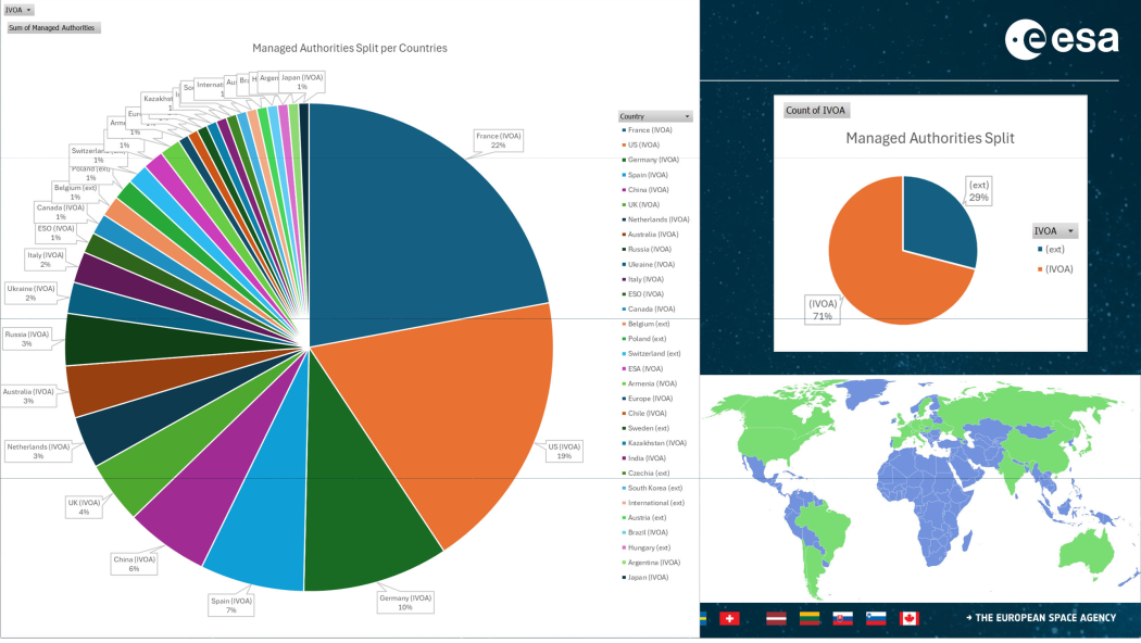
Given that, in Christophe's statistics talk, I was totally blown away by
the number of authorities and registries from Germany, given how small
GAVO is. Oh wow. In this graph of authorities in the VO we are the
dark green slice far at the bottom of the pie:
I will give you that, as usual with metrics, to understand what they
mean you have to know so much that you then don't need the metrics any
more. But
again there is an odd feeling of self-agency in that slide.
The next talk, Robert Nikutta's announcement of generic publishing
registry code, was – as already mentioned above –
particularly good news for me, because it let me
add something particularly straightforward into my overview of OAI-PMH
servers for VO use, and many data providers (those unwise enough to
not use DaCHS…) have asked for that.
For the rest of the session I entertained folks with the upcoming RFC of
VOResource 1.2 and the somewhat sad state of affairs in fulltext
seaches in the VO. Hence, I was too busy to report on how gracefully the
speaker made his points. Ahem.
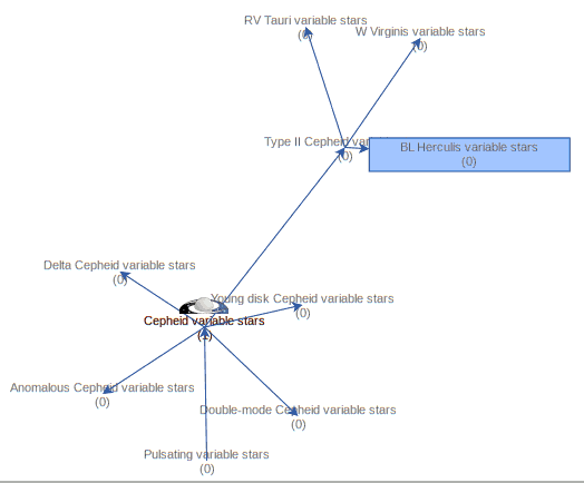
Semantics and Solar System (Saturday 16:30)
Ha! A session in which I don't talk. That's even more remarkable
because I'm the chair emeritus of the Semantics WG and the vice-chair of
the Solar Systems IG at the moment.
Nevertheless, my plan has been to sit back and relax. Except that some of
Baptiste's proposals for the evolution of the IVOA voacabularies
are rather controversial. I was therefore too busy to add to this
post again.
But at least there is hope to get rid of the ugly “(Obscure)” as the
human-readable label of the geo_app reference frame that entered that
vocabulary via VOTable; you see, this term was allowed in COOSYS/@system
since VOTable 1.0, but when we wrote the vocabulary, nobody who reviewed
it could remember what it meant. In this session, JJ finally
remembered. Ha! This will be a VEP soon.
It was also oddly gratifying to read this slide from Stéphane's talk on
fetching data from PDS4:
Lists like these are rather characteristic in a data publisher's
diary. Of course, I know that's true. But seeing it in public is
still gives me a warm feeling of comradeship.
Stéphane then went on to tell us how to make the
cool 67P images in TOPCAT (I had already mentioned those above when
I talked about the Exec report):
Operations (Sunday 10.00)
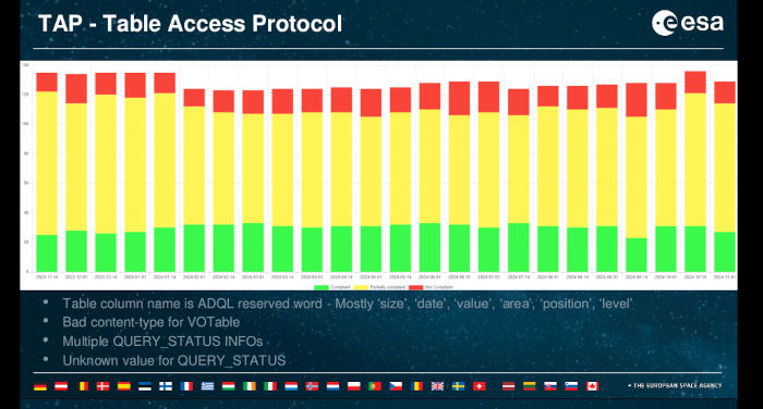
I am now in the session of the Operations IG, where Henrik is giving
the usual VO Weather Report. VO weather reports discuss how many of our
services are “valid” in the sense of “will work reasonably well with our
clients“. As usual for these kinds of metrics, you need to know quite a
bit to understand what's going on and how bad it is when a service is
“not compliant”. In particular for the TAP stats, things look a lot
bleaker than they actually are:
These assessments are based on stilts taplint, which is really fussy
(and rightly so). In reality, you can usually use even the red services
without noticing something is wrong. Except… if you are not doing
things quite right yourself.
That was the topic of my talk for Ops. It is another outcome of
this summer semester's VO course, where students were regularly
confused by diagnostics they got back. Of course, while on the learning
curve, you will see more such messages than if you are a researcher who
is just gently adapting some sample code. But anyway: Producing
good error messages is both hard and important. Let me quote my faux
quotes in the talk:
Writing good error messages is great art: Do not claim more than you
know, but state enough so users can guess how to fix it.
—Demleitner's first observation on error messages
Making a computer do the right thing for a good request usually is not
easy. It is much harder to make it respond to a bad request with a
good error message.
—Demleitner's first corollary on error messages
Later in the session there was much discussion about “denial of service
attacks” that services occasionally face. For us, that does not seem to
be malicious people in general, but people basically well-meaning but
challenged to do the right thing (read documentation, figure out
efficient ways to do what they want to do).
For instance, while far below DoS, turnitin.com was for a while
harvesting all VO registry records from some custom, HTML-rendering
endpoint every few days,
firing off 30'000 requests relatively expensive on my side (admittedly
because I have implemented that particular endpoint in the most lazy
fashion imaginable) in a rather short time. They could have done the
same thing using OAI-PMH with a single request that, no top, would
have taken up almost no CPU on my side. For the record, it seems
someone at turnitin.com has seen the light; at least they don't do that
mass harvesting any more for all I can tell (without actually checking
the logs). Still, with a
single computer, it is not hard to bring down your average VO server,
even if you don't plan to.
Operators that are going into “the cloud” (which is a thinly disguised
euphemism for “volunatrily becoming hostages of amazon.com”) or that are
severely “encouraged” to do that by their funding agencies have the
additional problem in that for them, indiscriminate downloads might quickly
become extremely costly on top. Hence, we were talking a bit about
mitigations, from HTTP 429 status codes (”too many requests“) to going
for various forms of authentication, in particular handing out API keys.
Oh, sigh. It would really suck if people ended up needing to get
and manage keys for all the major services. Perhaps we should have
VO-wide API keys? I already have a plan for how we could pull that
off…
Winding down (Monday 7:30)
The Interop concluded yesterday noon with reports from the working
groups and another (short) one from the Exec chair. Phewy. It's been
a straining week ever since ADASS' welcome reception almost exactly a
week earlier.
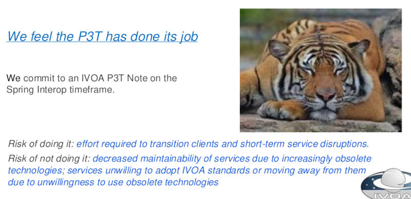
Reviewing what I have written here, I notice I have not even mentioned a
topic that pervaded several sessions and many of the chats on the
corridors: The P3T, which expands to “Protocol Transition Tiger Team”.
This was an informal working group that was formed because some adopters
of our standards felt that they (um: the standards)
are showing their age, in particular
because of the wide use of XML and because they do not always play well
with “modern” (i.e., web browser-based) “security” techniques, which of
course mostly gyrate around preventing cross-site information disclosure.
I have to admit that I cannot get too hung up on both points; I think
browser-based clients should be the exception rather than the norm in
particular if you have secrets to keep, and
many of the “modern” mitigations are little more than ugly hacks
(“pre-flight check“) resulting from the abuse of a system designed to
distribute information (the WWW) as an execution platform. But then
this ship has sailed for now, and so I recognise that we may need to
think a bit about some forms of XSS mitigations. I would still say
we ought to find ways that don't blow up all the sane parts of the VO
for that slightly insane one.
On the format question, let me remark that XML is not only well-thought
out (which is not surprising given its designers had the long history of
SGML to learn from) but also here to stay; developers will have to
handle XML regardless of what our protocols do. More to the point, it
often seems to me that people who say “JSON is so much simpler”
often mean “But it's so much simpler if my web page only talks to my
backend”.
Which is true, but that's because then you don't need to be
interoperable and hence don't have to bother with metadata for other
peoples' purposes. But that interoperability is what the IVOA is about.
If you were to write the S-expressions that XML encodes at its base in
JSON, it would be just as complex, just a bit more complicated because
you would be lacking some of XML's goodies from CDATA sections to
comments.
Be that as it may, the P3T turned out to do something useful: It tried
to write OpenAPI specifications for some of our protocols, and already
because that smoked out some points I would consider misfeatures
(case-insensitive parameter names for starters), that was certainly a
worthwhile effort. That, as some people pointed out, you can generate
code from OpenAPI is, I think, not terribly valuable: What code that
generates probably shouldn't be written in the
first place and rather be replaced by
some declarative input (such as, cough, OpenAPI) to a program.
But I will say that I expect OpenAPI specs to be a great help to
validators, and possibly also to implementors because they give some
implementation requirements in a fairly concise and standard form.
In that sense: P3T was not a bad thing. Let's see what comes out of it
now that, as Janet also reported in the closing session, the tiger is
sleeping:

![[RSS]](./theme/image/rss.png)
![A talk slide, with highlighted text: “Big Question: Why hasn't this [VOEvent] continued to serve the needs of various transient astrophysics communities?”](/media/2024/voevent-why-not.png)