![[RSS]](./theme/image/rss.png)
A Proposal for Persistent TAP Uploads
From its beginning, the IVOA's Table Access Protocol TAP has let users upload their own tables into the services' databases, which is an important element of TAP's power (cf. our upload crossmatch use case for a minimal example). But these uploads only exist for the duration of the request. Having more persistent user-uploaded tables, however, has quite a few interesting applications.
Inspired by Pat Dowler's 2018 Interop talk on youcat I have therefore written a simple implementation for persistent tables in GAVO's server package DaCHS. This post discusses what is implemented, what is clearly still missing, and how you can play with it.
If all you care about is using this from Python, you can jump directly to a Jupyter notebook showing off the features; it by and large explains the same things as this blogpost, but using Python instead of curl and TOPCAT. Since pyVO does not know about the proposed extensions, the code necessarily is still a bit clunky in places, but if something like this will become more standard, working with persistent uploads will look a lot less like black art.
Before I dive in: This is certainly not what will eventually become a standard in every detail. Do not do large implementations against what is discussed here unless you are prepared to throw away significant parts of what you write.
Creating and Deleting Uploads
Where Pat's 2018 proposal re-used the VOSI tables endpoint that every TAP service has, I have provisionally created a sibling resource user_tables – and I found that usual VOSI tables and the persistent uploads share virtually no server-side code, so for now this seems a smart thing to do. Let's see what client implementors think about it.
What this means is that for a service with a base URL of http://dc.g-vo.org/tap[1], you would talk to (children of) http://dc.g-vo.org/tap/user_tables to operate the persistent tables.
As with Pat's proposal, to create a persistent table, you do an http PUT to a suitably named child of user_tables:
$ curl -o tmp.vot https://docs.g-vo.org/upload_for_regressiontest.vot
$ curl -H "content-type: application/x-votable+xml" -T tmp.vot \
  http://dc.g-vo.org/tap/user_tables/my_upload
Query this table as tap_user.my_upload
The actual upload at this point returns a reasonably informative plain-text string, which feels a bit ad-hoc. Better ideas are welcome, in particular after careful research of the rules for 30x responses to PUT requests.
Trying to create tables with names that will not work as ADQL regular table identifiers will fail with a DALI-style error. Try something like:
$ curl -H "content-type: application/x-votable+xml" -T tmp.vot
  http://dc.g-vo.org/tap/user_tables/join
... <INFO name="QUERY_STATUS" value="ERROR">'join' cannot be used as an
  upload table name (which must be regular ADQL identifiers, in
  particular not ADQL reserved words).</INFO> ...
After a successful upload, you can query the VOTable's content as tap_user.my_upload:
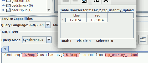
TOPCAT (which is what painted these pixels) does not find the table metadata for tap_user tables (yet), as I do not include them in the “public“ VOSI tables. This is why you see the reddish syntax complaints here.
I happen to believe there are many good reasons for why the volatile and quickly-changing user table metadata should not be mixed up with the public VOSI tables, which can be several 10s of megabytes (in the case of VizieR). You do not want to have to re-read that (or discard caches) just because of a table upload.
If you have the table URL of a persistent upload, however, you inspect its metadata by GET-ting the table URL:
$ curl http://dc.g-vo.org/tap/user_tables/my_upload | xmlstarlet fo
<vtm:table [...]>
  <name>tap_user.my_upload</name>
  <column>
    <name>"_r"</name>
    <description>Distance from center (RAJ2000=274.465528, DEJ2000=-15.903352)</description>
    <unit>arcmin</unit>
    <ucd>pos.angDistance</ucd>
    <dataType xsi:type="vs:VOTableType">float</dataType>
    <flag>nullable</flag>
  </column>
  ...
– this is a response as from VOSI tables for a single table. Once you are authenticated (see below), you can also retrieve a full list of tables from user_tables itself as a VOSI tableset. Enabling that for anonymous uploads did not seem wise to me.
When done, you can remove the persistent table, which again follows Pat's proposal:
$ curl -X DELETE http://dc.g-vo.org/tap/user_tables/my_upload
Dropped user table my_upload
And again, the text/plain response seems somewhat ad hoc, but in this case it is somewhat harder to imagine something less awkward than in the upload case.
If you do not delete yourself, the server will garbage-collect the upload at some point. On my server, that's after seven days. DaCHS operators can configure that grace period on their services with the [ivoa]userTableDays setting.
Authenticated Use
Of course, as long as you do not authenticate, anyone can drop or overwrite your uploads. That may be acceptable in some situations, in particular given that anonymous users cannot browse their uploaded tables. But obviously, all this is intended to be used by authenticated users. DaCHS at this point can only do HTTP basic authentication with locally created accounts. If you want one in Heidelberg, let me know (and otherwise push for some sort of federated VO-wide authentication, but please do not push me).
To just play around, you can use uptest as both username and password on my service. For instance:
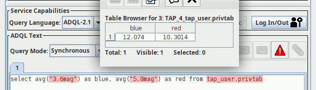
  $ curl -H "content-type: application/x-votable+xml" -T tmp.vot \
  --user uptest:uptest \
  http://dc.g-vo.org/tap/user_tables/privtab
Query this table as tap_user.privtab
In recent TOPCATs, you would enter the credentials once you hit the Log In/Out button in the TAP client window. Then you can query your own private copy of the uploaded table:
There is a second way to create persistent tables (that would also work for anonymous): run a query and prepend it with CREATE TABLE. For instance:
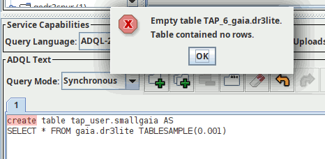
The “error message” about the empty table here is to be expected; since this is a TAP query, it stands to reason that some sort of table should come back for a successful request. Sending the entire newly created table back without solicitation seems a waste of resources, and so for now I am returning a “stub” VOTable without rows.
As an authenticated user, you can also retrieve a full tableset for what user-uploaded tables you have:
$ curl --user uptest:uptest http://dc.g-vo.org/tap/user_tables | xmlstarlet fo
<vtm:tableset ...>
  <schema>
    <name>tap_user</name>
    <description>A schema containing users' uploads. ...  </description>
    <table>
      <name>tap_user.privtab</name>
      <column>
        <name>"_r"</name>
        <description>Distance from center (RAJ2000=274.465528, DEJ2000=-15.903352)</description>
        <unit>arcmin</unit>
        <ucd>pos.angDistance</ucd>
        <dataType xsi:type="vs:VOTableType">float</dataType>
        <flag>nullable</flag>
      </column>
      ...
    </table>
    <table>
      <name>tap_user.my_upload</name>
      <column>
        <name>"_r"</name>
        <description>Distance from center (RAJ2000=274.465528, DEJ2000=-15.903352)</description>
        <unit>arcmin</unit>
        <ucd>pos.angDistance</ucd>
        <dataType xsi:type="vs:VOTableType">float</dataType>
        <flag>nullable</flag>
      </column>
      ...
    </table>
  </schema>
</vtm:tableset>
Open Questions
Apart from the obvious question whether any of this will gain community traction, there are a few obvious open points:
Indexing. For tables of non-trivial sizes, one would like to give users an interface to say something like “create an index over ra and dec interpreted as spherical coordinates and cluster the table according to it”. Because this kind of thing can change runtimes by many orders of magnitude, enabling it is not just some optional embellishment.
On the other hand, what I just wrote already suggests that even expressing the users' requests in a sufficiently flexible cross-platform way is going to be hard. Also, indexing can be a fairly slow operation, which means it will probably need some sort of UWS interface.
Other people's tables. It is conceivable that people might want to share their persistent tables with other users. If we want to enable that, one would need some interface on which to define who should be able to read (write?) what table, some other interface on which users can find what tables have been shared with them, and finally some way to let query writers reference these tables (tap_user.<username>.<tablename> seems tricky since with federated auth, user names may be just about anything).
Given all this, for now I doubt that this is a use case sufficiently important to make all the tough nuts delay a first version of user uploads.
Deferring destruction. Right now, you can delete your table early, but you cannot tell my server that you would like to keep it for longer. I suppose POST-ing to a destruction child of the table resource in UWS style would be straightforward enough. But I'd rather wait whether the other lacunae require a completely different pattern before I will touch this; for now, I don't believe many persistent tables will remain in use beyond a few hours after their creation.
Scaling. Right now, I am not streaming the upload, and several other implementation details limit the size of realistic user tables. Making things more robust (and perhaps scalable) hence will certainly be an issue. Until then I hope that the sort of table that worked for in-request uploads will be fine for persistent uploads, too.
Implemented in DaCHS
If you run a DaCHS-based data centre, you can let your users play with the stuff I have shown here already. Just upgrade to the 2.10.2 beta (you will need to enable the beta repo for that to happen) and then type the magic words:
dachs imp //tap_user
It is my intention that users cannot create tables in your DaCHS database server unless you say these words. And once you say dachs drop --system //tap_user, you are safe from their huge tables again. I would consider any other behaviour a bug – of which there are probably still quite a few. Which is why I am particularly grateful to all DaCHS operators that try persistent uploads now.
| [1] | As already said in the notebook, if http bothers you, you can write https, too; but then it's much harder to watch what's going on using ngrep or friends. |