2024-02-23
Markus Demleitner
One of the more exciting promises of the Virtual Observatory was global
dataset discovery: You say “Give me all spectra of object X that there
are“, and the computer relates that request to all the services that
might have applicable data. Once the results come in, they are merged into some
uniformly browsable form.
In the early VO, there were a few applications that let you do this; I
fondly remember VODesktop. As the VO grew and diversified, however,
this became harder and harder, partly because there were more and more
services, partly because there were more protocols through which to
publish data. Thus, for all I can see, there is, at this point, no
software that can actually query all services plausibly serving, say,
images or spectra in the VO.
I have to say that writing such a thing is not for the faint-hearted,
either. I probably wouldn't have tackled it myself unless the pyVO
maintainers had made it an effective precondition for cleaning up the
pyVO Servicetype constraint.
But they did, and hence as a model I finally wrote some code to do
all-VO image searches using all of SIA1, SIA2, and obscore, i.e., the
two major versions of the Simple Image Access Protocol plus Obscore
tables published through TAP services. I actually have already
reported in Tucson on some preparatory work I did last
summer and named a few problems:
- There are too many services to query on a regular basis, but filtering
them would require them to declare their coverage; far too many still don't.
- With the current way of registering obscore tables, there is no way to
know their coverage.
- One dataset may be availble through up to three protocols on a single
host.
- SIA1 does not even let you constrain time and spectrum.
Some of these problems I can work around, others I can try to fix. Read
on to find out how I fared so far.
The pyVO API
Currently, the development happens in pyVO PR #470. While it is
still a PR, let me point you to temporary pyVO docs on the proposed
pyvo.discover module – of course, all of this is for review and probably
not in the shape it will remain in.
With the recent release of pyVO 1.6, what is described here is
actually available in the release (or by checking out the main branch
of the repository).
To quote from there, the basic usage would be something like:
from pyvo import discover
from astropy import units as u
from astropy import time

datasets, log = discover.images_globally(
  space=(339.49, 3.1, 0.1),
  spectrum=650*u.nm,
  time=(time.Time('1995-01-01'), time.Time('1995-12-31')))
At this point, only a cone is supported as a space constraint, and only
a single point in spectrum. It would certainly be desirable to be more
flexible with the space constraint, but given the capabilities of the
various protocols, that is hard to do. Actually, even with the plain
cone Obscore (i.e., ironically, the most powerful of the discovery
protocols covered here) currently results in an implementation that
makes me unhappy: ugly, slow, and wrong. This is requires a longer
discussion; see Appendix: Optionality Considered Harmful.
datasets at this point is a list of, conceputally, Obscore records.
Technically, the list contains
instances of a custom class ImageFound, which have
attributes named after the Obscore columns. In case you have doubts
about the Semantics of any column, the Obscore specification is there
to help. And yes, you can argue we should create a single astropy table
from that list. You are probably right.
PyVO adds an extra column over the mandatory obscore set,
origin_service. This contains the IVOA identifier (IVOID) of the service at
which the dataset was found. You have probably seen IVOIDs before: they
are URIs with a scheme of ivo:. What you may not know: these things
actually resolve, specifically to registry resource records. You can do
this resolution in a web browser: Just prepend https://dc.g-vo.org/I/
to an IVOID and paste the result into the address bar. For instance, my
Obscore table has the IVOID
ivo://org.gavo.dc/__system__/obscore/obscore; the link below the
IVOID leads you to an information page, which happens to be the
resource's Registry record formatted with a bit of XSLT. A somewhat
more readable but less informative rendering is available when you
prepend https://dc.g-vo.org/LP/ (“landing page”).
The second value returned from discover.images_globally is a list of
strings with information on how the global discovery progressed. For
now, this is not intended to be machine-readable. Humans can figure out
which resources were skipped because other services already cover their
data, which services yielded how many records, and which services
failed, for instance:
Skipping ivo://org.gavo.dc/lswscans/res/positions/siap because it is served by ivo://org.gavo.dc/__system__/obscore/obscore
Skipping ivo://org.gavo.dc/rosat/q/im because it is served by ivo://org.gavo.dc/__system__/obscore/obscore
Obscore GAVO Data Center Obscore Table: 2 records
SIA2 The VO @ ASTRON SIAP Version 2 Service: 0 records
SIA2 ivo://au.csiro/casda/sia2 skipped: ReadTimeout: HTTPSConnectionPool(host='casda.csiro.au', port=443): Read timed out. (read timeout=20)
SIA2 CADC Image Search (SIA): 0 records
SIA2 European HST Archive SIAP service: 0 records
...
(On the skipping, see Relationships below). I consider this crucial
provenance, as that lets you assess later what you may have missed.
When you save the results, be sure to save these, too.
A feature that will presumably (see Inclusivity for the reasons for
this expectation) be important at least for a few years is that you can
pass the result of a Registry query, and pyVO will try to find services
suitable for image discovery on that set of resources.
A relatively straightforward use case for that is global obscore
discovery. This would look like this:
from pyvo import discover
from pyvo import registry
from astropy import units as u
from astropy import time

def say(discoverer, s):
        print(s)

datasets, log = discover.images_globally(
  space=(274.6880, -13.7920, 1),
  time=(time.Time('1995-01-01'), time.Time('1995-12-31')),
  services=registry.search(registry.Datamodel("obscore")),
  watcher=say)
The watcher thing lets you, well, watch the progress of the
discovery; it receives an instance of the discoverer -- this is so you
can abort a discoverer's activities from within some UI --
and the human-readable string to display or process in some other way.
A UI
To get an idea whether this API might one day work for the average
astronomer, I have written a Tkinter-based GUI to global image discovery
as it is now: tkdiscover (only available from github at this point).
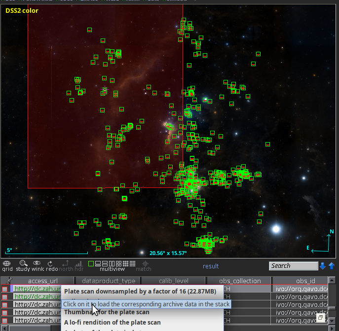
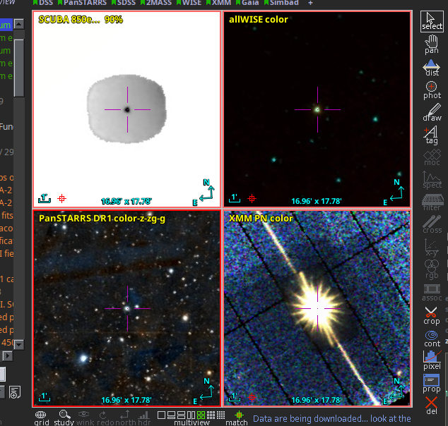
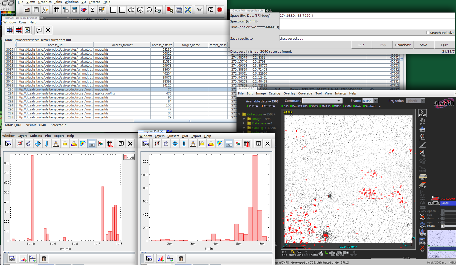
This is what a session with it might look like:
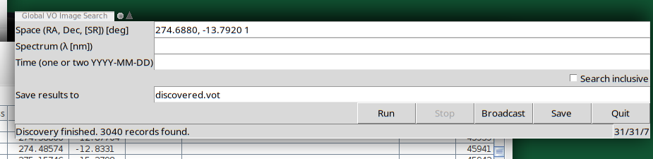
The actual UI is in the top right: A plain window in which you can
configure a global discovery query by straightfoward serialisations of
discover.images_globally's arguments:
- Space (currently, a cone in RA, Dec, and search radius, separated by
whitespace of commas)
- Spectrum (currently, a single point as a wavelength in metres)
- Time (currently, either a single point in time – which probably is
rarely useful – or an interval, to be entered as civil DALI dates
- Inclusivity.
When you run this, this basically calls discover.images_globally
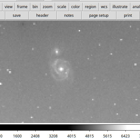
and lets you know how it is progressing. You can click Broadcast
(which sends the current result to all VOTable clients on the
SAMP bus) or Save at any time and inspect how discovery is
progressing. I predict you will want to do that, because querying
dozens of services will take time.
There is also a Stop button that aborts the dataset search (you will
still have the records already found). Note that the Stop button will
not interrupt running network operations, because the network library
underneath pyVO, requests, is not designed for being interrupted.
Hence, be patient when you hit stop; this may take as long as the
configured timeout (currently is 20 seconds) if the service hangs or has
to do a lot of work. You can see that tkdiscover has noticed your stop
request because the service counter will show a leading zero.
Service counter? Oh, that's what is at the bottom right of the window.
Once service discovery is done, that contains three numbers: The number
of services to query, the number of services queried already, and the
number of services that failed.
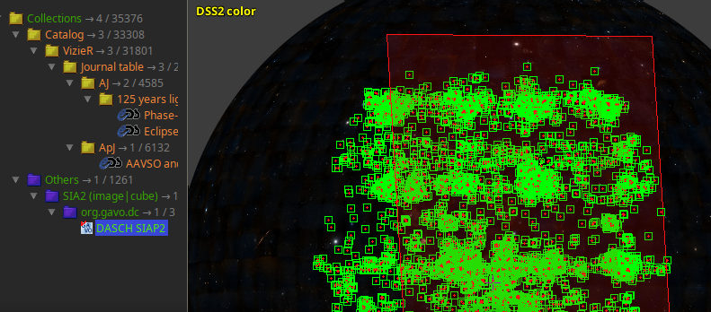
The table contains the obscore records described above, and the log
lines are in the discovery_log INFO. I will give you that this is
extremely unreadable in particular in TOPCAT, which normalises the line
separators to plain whitespace. Perhaps some other representation of
these log lines would be preferable: A PARAM with a char[][] (but
VOTable still is terrible with arrays of variable-length strings)? Or a
separate table with char[*] entries?
Inclusivity
I have promised above I'd explain the “Inclusive” part in both the pyVO
API and the Tk UI. Well, this is a bit of a sad story.
All-VO-queries take time. Thus, in pyVO we try to only query services
that we expect serve data of interest. How do we arrive at expectations
like that? Well, quite a
few records in the Registry by now declare their coverage in space and
time (cf. my 2018 post for details).
The trouble is: Most still don't. The checkmark at inclusive
decides whether or not to query these “undecidable” services. Which
makes a huge difference in runtime and effort. With the pre-configured
constraints in the current prototype (X-Ray images a degree around
274.6880, -13.7920 from the year 1995), we currently discover three
services (of which only one actually needs to be queried) when
inclusive is off. When it is on, pyVO will query a whopping 323
services (today).
The inclusivity crisis is particularly bad with Obscore tables because
of their broken registration pattern; I can say that so bluntly because
I am the author of the standard at fault, TAPRegExt. I am preparing a
note with a longer explanation and proposals for fixing matters –
<cough> follow me on github –, but in all brevity: Obscore data is
discovered using something like a flag on TAP services. That is bad
because the TAP services usually have entriely different metadata from
their Obscore table; think, in particular, of the physical coverage that
is relevant here.
It will be quite a bit of effort to get the data providers to do the
Registry work required to improve this situation. Until that is done,
you will miss Obscore tables when you don't check inclusive (or
override automatic resource selection as above) – and if
you do check inclusive, your discovery runs will take something like a
quarter of an hour.
Relationships
In general, the sheer number of services to query is the Achilles' heel
in the whole plan. There is nothing wrong with having a machine query 20
services, but querying 200 is starting to become an effort.
With multi-data collection services like Obscore (or collective SIA2
services), getting down to a few dozen services globally for a
well-constrained search is actually not unrealistic; once all resources
properly declare their coverage, it is not very likely that more than 20
institutions worldwide will have data in a credibly small region of
space, time, and spectrum. If all these run collective services and
properly declare the datasets to be served by them, that's our
20-services global query right there.
However, pyVO has to know when data contained in a resource is actually
queriable by a collective service. Fortunately, this problem has
already been addressed in the 2019 endorsed note on Discovering Data
Collections Within Services: Basically, the individual resource
declares an IsServedBy relationship to the collective service. PyVO
global discovery already looks at these. That is how it could figure
out these two things in the sample log given above:
Skipping ivo://org.gavo.dc/lswscans/res/positions/siap because it is served by ivo://org.gavo.dc/__system__/obscore/obscore
Skipping ivo://org.gavo.dc/rosat/q/im because it is served by ivo://org.gavo.dc/__system__/obscore/obscore
But of course the individual services have to declare these
relationships. Surprisingly many already do, as you can observe
yourself when you run:
select ivoid, related_id from
rr.relationship
natural join rr.capability
where
standard_id like 'ivo://ivoa.net/std/sia%'
and relationship_type='isservedby'
on your favourite RegTAP endpoint (if you have no preferences, use mine:
http://dc.g-vo.org/tap). If you have collective services and run
individual SIA services, too, please run that query, see if you are in
there, and if not, please declare the necessary relationships. In case
you are unsure as to what to do, feel free to contact me.
Future Directions
At this point, this is a rather rough prototype that needs a lot of
fleshing out. I am posting this in part to invite the more adventurous
to try (and break) global discovery and develop further ideas.
Some extensions I am already envisaging include:
Write a similar module for spectra based on SSAP and Obscore. That
would then probably also work for time series and similar 1D data.
Do all the Registry work I was just talking about.
Allow interval-valued spectral constraints. That's pretty
straightforward; if you are looking for some place to contribute code,
this is what I'd point you to.
Track overflow conditions. That should also be simple, probably just
a matter of perusing the pyVO docs or source code and then
conditionally produce a log entry.
Make an obscore s_region out of the SIA1 WCS information. This should
also be easy – perhaps someone already has code for that that's tested
around the poles and across the stitching line? Contributions are
welcome.
Allow more complex geometries to define the spatial region of
interest. To keep SIA1 viable in that scenario it would be
conceivable to compute a bounding box for SIA1 POS/SIZE
and do “exact” matching locally on the coarser SIA1 result.
Enable multi-position or multi-interval constraints. This pretty
certainly would exclude SIA1, and, realistically, I'd probably only
enable Obscore services with TAP uploads with this. With those
constraints, it would be rather straightforward.
Add SODA support: It would be cool if my ImageFound had a way to
say “retrieve data for my RoI only”. This would use SODA and datalink
to do server-side cutouts where available and do the cut-out locally
otherwise. If this sounds like rocket science: No, the standards for
that are actually in place, and pyVO also has the necessary support
code. But still the plumbing is somewhat tricky, partly also because
pyVO's datalink API still is a bit clunky.
Going async? Right now, we civilly query one service after the other,
waiting for each result before proceeding to the next service. This
is rather in line with how pyVO is written so far.
However, on the network side for many years asynchronous programming
has been a very successful paradigm – for instance, our DaCHS package
has been based on an async framework from the start, and Python itself
has growing in-language support for async, too.
Async allows you to you fire off a network request and forget about it
until the results come back (yes, it's the principle of async TAP,
too). That would let people run many queries in parallel, which in
turn would result in dramatically reduced waiting times, while we can
rather easily ensure that a single client will not overflow any
server. Still, it would be handing a fairly powerful tool into
possibly unexperienced hands… Well: for now there is no need to decide
on this, as pyVO would need rather substantial upgrades to support async.
Appendix: Optionality Considered Harmful
The trouble with obscore and cones is a good illustration of the traps
of attempting to fix problems by adding optional features. I currently
translate the cone constraint on Obscore using:
"(distance(s_ra, s_dec, {}, {}) < {}".format(
  self.center[0], self.center[1], self.radius)
+" or 1=intersects(circle({}, {}, {}), s_region))".format(
  self.center[0], self.center[1], self.radius))
which is all of ugly, presumably slow, and wrong.
To appreciate what is going on, you need to know that Obscore has two
ways to define the spatial coverage of an observation. You can give its
“center” (s_ra, s_dec) and something like a rough radius
(s_fov), or you can give some sort of geometry (e.g., a polygon:
s_region). When the standard was written, the authors wanted to
enable Obscore services even on databases that do not know about
spherical geometry, and hence s_region is considered rather
optional. In consequence, it is missing in many services. And even the
s_ra, s_dec, s_fov combo is not mandatory non-null, so you
are perfectly entitled to only give s_region.
That is why there are the two conditions or-ed together (ugly) in the
code fragment above. 1=intersects(circle(.), s_region) is the
correct part; this is basically how the cone is interpreted in SIA1,
too. But because s_region may be NULL even when s_ra and
s_dec are given, we also need to do a test based on the center
position and the field of view. That rather likely makes things slower,
possibly quite a bit.
Even worse, the distance-based condition actually is wrong. What I really
ought to take into account is s_fov and then do something like
distance(.) < {self.radius}+s_fov, that is, the dataset position
need only be closer than the cone radius plus the dataset's FoV
(“intersects”). But that would again produce a lot of false negatives
because s_fov may be NULL, too, and often is, after which the whole
condition would be false.
On top of that, it is virtually impossible that such an expression would
be evaluated using an index, and hence with this code in place, we would
likely be seqscanning the entire obscore table almost every time – which
really hurts when you have about 85 Million records in your Obscore
table (as I do).
The standard could immediately have sanitised all this by saying: when
you have s_ra and s_dec, you must also give a non-empty
s_fov and s_region. This is a classic case for where a MUST
would have been necessary to produce something that is usable without
jumping through hoops. See my post on Requirements and Validators on
this blog for a longer exposition on this whole matter.
I'm not sure if there is a better solution than the current “if the
operators didn't bother with s_region, the dataset's FoV will be
ignored“. If you have good ideas, by all means let me know.

![[RSS]](./theme/image/rss.png)