![[RSS]](./theme/image/rss.png)
DaCHS 2.9 is out
Our VO server package DaCHS almost always sees two releases per year, each time roughly after the Interops[1]. So, with the Tucson Interop over, it's time for DaCHS 2.9, and this is the traditional what's new post.
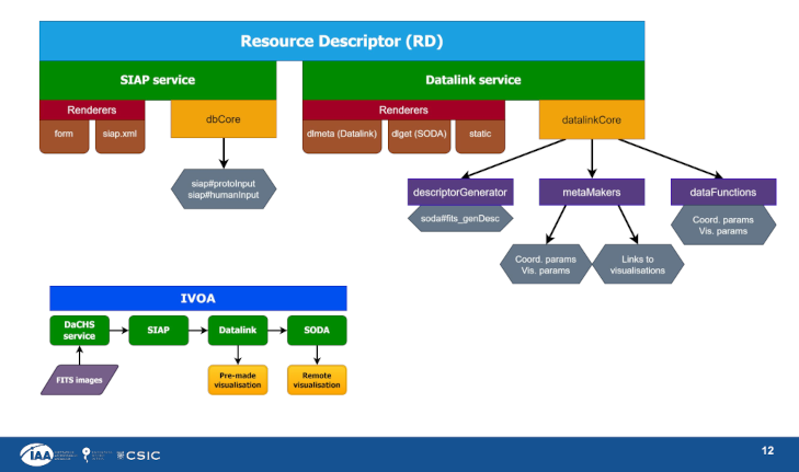
Data Origin – the big headline for this release could be “curation”, in that three upcoming standardoid entities in that field are prototyped in 2.9. One is Data Origin, which is a note on how to embed some very basic provenance information into VOTables.
This is going to help your users figure out how they came up with a VOTable when the referee has clever questions about the paper they submitted half a year earlier. The good news is: if you defined your metadata in your RD with sufficient care, with DaCHS 2.9 you will automatically do Data Origin.
Feed your D links – another curation-related new thing in DaCHS is an implementation of what will hopefully be known as BibVO in the future. At this point, it is an unpublished note on Github. In essence, the purpose is to feed bibliographic services – and in particular the ADS – “D links”, i.e., links from publications to data. A part of this works automatically (the source metadatum), but the more advanced biblinks need a bit of manual intervention.
If you even have, say, an observatory bibliography consisting pairs of papers and data used by these papers, you will probably have to write a handful of code. See biblinks in the reference documentation for details if any of this sounds as if it could apply to you. In this context, I have also enabled passing multiple accrefs to the /get endpoint. Users will then receive a tar file of the referenced data products.
altIdentifiers in relationships – still in the bibliographic realm, VOResource 1.2 will (almost certainly) let you set altIdentifiers, in particular DOIs, when you declare relationships to other resources. That is probably of interest in particular when you want to declare relationships to things outside of the VO to services like b2find that themselves do not understand ivoids. In that situation, you would write something like:
Cites: Some external thing
Cites.altIdentifier: doi:10.fake/123412349876
in a <meta> tag in your RD.
json columns – postgresql has the very tempting and apparently all-powerful json type; it lets you stick complex structures into database columns and thus apparently relieve you of all the tedious tasks of designing database tables and documenting metadata.
Written like this, you probably notice it's a slippery slope at best. Still, there are some non-hazardous uses for such columns, and thus you can now say type="json" or (probably preferably) type="jsonb" in column definitions. You can feed these columns with dicts, lists or JSON literals in strings. Clients will receive both of them as JSON string literals in char[*] FIELDs with an xtype of json. Neither astropy nor TOPCAT do anything with that xtype yet, but I expect that will change soon.
Copy coverage – sometimes two resources have the same spatial (and potentially temporal and spectral) coverage. Since obtaining the coverage is an expensive operation, it would be nice to be able to say “aw, look at that other resource and take its coverage.” The classic example in DaCHS is the system-wide SIAP2 service that really is just a parametric wrapper around obscore. In such cases, you can now say something like:
<coverage fallbackTo="__system__/obscore"/>
– and //siap2 already does. That's one more reason to occasionally run dachs limits //obscore if you offer an obscore table.
First VOTable row in tests – if you have calls to getFirstVOTableRow in regression tests (you have regression tests, right?) that return multiple rows, these will fail now until you also pass rejectExtras=False to that call. I've had regressions that were hidden by the function's liberal acceptance of extra rows, and it's too simple to produce unstable tests (that magically succeed and fail depending to the current state of the database) with the old behaviour. I hence hope for your sympathy and understanding in case I broke one of your tests.
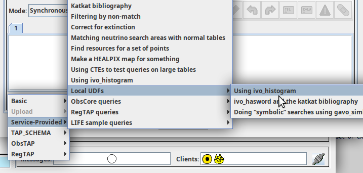
ADQL extensions – there is now arr_count to complement the array extension added in 2.7. Also, our custom UDFs transform, normal_random, to_jd, to_mjd, and simbadpoint now have a prefix of ivo_ rather than the previous gavo_. In order not to break existing queries, DaCHS will still accept the gavo_-prefixed names for the forseeable future, but it will no longer advertise them.
Minor fixes – as usual, there are many minor bug fixes and improvements, the most visible of which is probably that DaCHS now correctly handles literal + chars in multipart-encoded (”uploads”) requests again; that was broken in 2.8 after the removal of the dependency on python's CGI module. Also, MOC-valued columns can now be serialised into non-VOTable formats like JSON or CSV.
If you have been using DaCHS' built-in HTTPS support, certain clients may have rejected its certificates. That was because we were pulling an expired intermediate certificate from letsencrypt. If you don't understand what I was just saying, don't worry. If you do understand that and know a good way to avoid this kind of calamity in the future, I'm grateful for advice.
VCS move – when DaCHS was born, using the venerable subversion for version control was considered reputable. These days, fewer and fewer people can still deal with that, and thus I have moved the DaCHS source code into a git repository: https://gitlab-p4n.aip.de/gavo/dachs/.
I hear you moan “why not github?” Well: don't get me started unless you are prepared to listen to a large helping of proselytising. Suffice it to say that we in academia invented the internet (for all intents and purposes) and it's a shame that we now rely so much on commercial entities to provide our basic services (and then without paying them, as a rule, which is always a dangerous proposition towards commercial entities).
Anyway: Feel free to use that service's bug tracker; we try to find ways to let you log in there without undue hardship, too.
At this point, I customarily urge: don't wait, upgrade. If you have our Debian repository enabled, apt update && apt upgrade should do the trick, except if you missed our announcement on dachs-users that our repository key has changed. If you have not updated it, please have a look at our repo page to see what needs to be done. Sorry about this, but our old 1024D key was being frowned upon, so we had to do something.
Unless you are an old hand and have upgraded many times before, let me recommend a quick glance at our upgrading guide before doing the actual upgrade.
| [1] | The reason we wait for the Interops is that we are generally promising to put something into DaCHS at or around these conferences. This time, the preliminary support for json-typed database columns is an example for that. |