![[RSS]](./theme/image/rss.png)
At the Bologna Interop
As I usually do at Interops, I plan to give a few impressions from the Virtual Observatory's semiannual get-together on this blog, updating as we go. This time, it's about the May 2023 Bologna Interop.
After six „virtual“ Interops (the last one in October 2022), this is the first one with actual people and, most importantly, an actual coffee break table. Attempts to replace that with gathertown, I have to say, never really panned out, so I'm looking forward to pushing ahead many of the small things that make a project like the VO tick, and do that with less effort than try and get people into telecons.
Also, it's my last Interop as chair of the Semantics Working Group – to prevent informal hierarchies as well as possible, there's a limit of four years in a single IVOA position, and my four years as the herder of meanings are now over. So, the Bologna Semantics Session will be the last one I will chair. Will you do me a favour and attend? Since the conference is hybrid, you can even do that if you are not in town.
2023-05-09, 10:00
I approached this morning's Science Platform Plenary with a fair amount of apprehension because I'm always worried that these platforms actually appear so attractive to management because they are the old silos management knows. For instance, people would go back to write software for their data specifically and no one could be blamed for “wasting“ money on software useful to others.
Sure, custom and tailored software is faster to do, and the resulting lock-in perhaps even helps getting shiny metrics for a while, but the results are also much faster to break, not to mention interoperability goes down the drain, it's a big exercise in exclusion, and of course everyone re-implementing about the same thing every time is a gigantic waste of money and, worse, human effort.
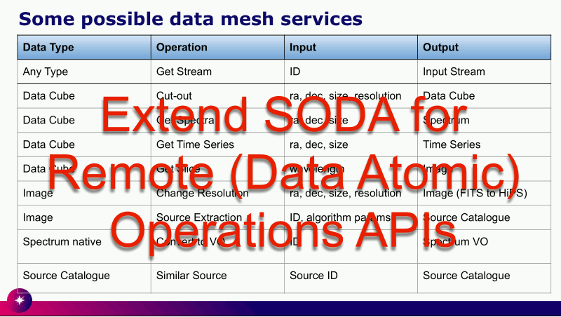
Slide 13 from Jesus' talk. Rights his.
Fortunately, most of the talks did not aggravate these concerns. On the contrary, most of what I saw was fairly generic compute platforms that very credibly strive to be open, both on getting things in and getting things out.
But I'll not deny that what I particularly liked was Jesus Salgado's distinctly un-platformy proposals for extending SODA (slide 13) – most of the operations envisaged sound very useful, sensible, and doable, and I will certainly put them into DaCHS if someone (cough else) works them out.
The only really alarming thing I heard in the platforms session was the term “multi-factor authentication“.
Come on, none of what we're doing here is the sort of thing where anything major would break if someone pilfered credentials. Please, please let's be reasonable. There's a lot less harm done if someone runs a few CPU hours on someone else's account than if humans were forced to copy many digits from one device to another device all the time[1].
Don't get me wrong: There are places where 2FA may be a good idea, in particular when other peoples' personal data is concerned. I'm just saying that most of the time, 2FA causes more annoyance than the occasional pilfered credential would (and that you shouldn't process other peoples' personal data without a really strong reason in the first place).
2023-05-09, 17:00
A personal highlight of every Interop for me as a Registry geek is of course the session of the Registry WG, which today featured two talks by yours truly. However, it opened with a slightly humbling piece by Hendrik Heinl on how unsatisfying it is to discover time series in the current VO. It would have been badly humbling if it hadn't highlighted why several of the things I've been after for many years matter, most of all the move to data discovery I have talked about here before.
Of my two talks, one was an abridged and perhaps a bit more entertaining version of my recent blog post on the various sorts of lint I find in the VO Registry. The other was very dry fare on standards development; only look at it if you're into evolving VOResource and its extensions, and I'm afraid I have to say about as much on Renaud's contribution on some incremental changes to StandardsRegExt, which in itself works pretty much exclusively behind the scenes. Suffice it to say that even in the VO there are those little thankless jobs.
2023-05-10 16:00
Phewy. Another two talks down, one to go. In the session informally called DOI I (where DOI here is a Digital Object Identifier, in our case almost always managed through DataCite), I reminded everyone that if they have an IVOID (in plain English: are in the VO Registry), they can improve their citeability dramatically by getting themselves a DOI using voidoi (which of course only is interesting if you cannot or do not want to mint your resource's DOI in some other way).
Let me mount a soapbox here for a moment: I'm caring about DOIs because I want paper authors to be able to cite data in a way that lets people find the resources used. That in the case of a DOI the reference is machine-readable to me is a liability rather than an advantage, since it makes it even easier to come up with metrics. And metrics, I claim, are almost always a bad thing, either masking agendas that should be made explicit or, worse and more typical, making matters worse accidentally – which is almost inevitable as soon as people start gaming the metrics, which in turn is almost inevitable when you threaten their livelihoods using metrics.
Given that, it was not easy keeping quiet and not starting to argue points to that effect (which I'll gladly do here if anyone gives me an excuse to do so) during much of the second DOI session. Let me at least make one point to any funders possibly venturing here: Persistent identifiers to data don't make persistent institutions keeping the data obsolete.
Such persistent institutions also have a critical role in curating the metadata going into the PIDs, a point driven home in Gus' talk; look at slide 15 for impressions of the sort of desasters happening when you create citations from DataCite records encountered in the wild. In my assumed role as a Registry janitor (as per this recent post) I had complete empathy with Gus.
My second talk this morning I again gave in the wonderful large auditorium (a real treat for a limelight hog like me): I talked about the hairy problems raised by major version steps in protocols. There was not too much discussion on this – less than I had hoped for, really, in particular later during the lunch break –, but having presented the problem in front of this kind of audience, I'm now rather sure the right way to proceed is what's Option I in my talk: deprecate servicetype='image'. The sort of global discovery that was envisaged to be enabled by servicetype constraints probably needs to be handled in a proper function hiding the gory details from the users.
2023-05-11, 12:30
This morning I had the last session in my term as the chair of the Semantics working group, featuring talks reporting on the progress of various semantic artefacts by different people; whether or not it's justified, I feel some satisfaction seeing this sort of activity that I'd take as the sign of a mature working group operating.
Me, on the other hand, talked quite a bit on an entirely maverick topic: Linked Data in VOTable. As I point out in the talk, in the one place we are using RDFa (which I identify with the buzzword “linked data“ for the purposes of this talk) in the VO it's a big success (TAP examples, which use RDFa over XHTML). Perhaps we should have more of that?
The obvious place to add RDFa to VO stuff would be our central container format VOTable, which conveniently is based on XML, and hence existing RDFa tooling is immediately applicable when we add a few RDFa attributes to a few VOTable elements. I proved that with some examples and three lines of pyrdfa code and was sort-of happy with getting nice, Turtle-formatted RDF triples out of very lightly annotated VOTables.
However, if you have followed the pyrdfa link, you may have seen the main argument against the whole effort:
This repository has been archived by the owner on Jun 21, 2022. It is now read-only.
It would seem that RDFa within XML-derived formats is not a terribly active topic these days. If that's true, then effort from the VO side to be interoperable with this part of the outside world would be largely wasted – that outside world might very well be smaller than the VO itself now. On the other hand, if I look at Linked Open Vocabularies, it would seem that there are communities using RDF as such very actively, and some of these vocabularies we could very well reuse.
And then there is a problem I couldn't figure out that may be a good test case for using ChatGPT on technical questions (feel free to try): “How do I make an RDF resource out of element content in RDFa?“ In case that's too dense a question: What I'd like to do is some RDFa markup such that:
<INFO property="doap:homepage"
  magic-attribute="magic-value"
  >http://foo.bar"</INFO>
works out to:
<> doap:homepage <http://foo.bar>
in Turtle (note the angle brackets rather than quotes, indicating we are talking about an RDF resource rather than a literal that happens to look like a URI). Can't be hard, can it?
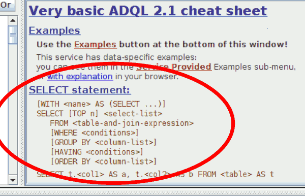
New in TOPCAT: If it senses that a service understands common table expressions, it will inform you accordingly on its ADQL cheat sheet.
Oh, and then I'd like to add an impression from the Apps/Ops session late on Wednesday, where I simply have to hand out the tasteful-application-of-standards award to Mark Taylor. In his news from TOPCAT report he described how based on whether or not the capabilities of a TAP service say its ADQL supports CTEs (“WITH”) he changes his cheat sheet to show or hide the optional with clause as shown in the figure above.
Sure: That's a real small detail. But sometimes it's small details like this that make the difference between folks puzzling how to do a seemingly simple thing (as I am still on the resourcification of element content in RDFa) and them realising there is an elegant solution to what they're trying to do.
2023-05-13 11:00
The Interop ended yesterday morning, and now I'm returning home with about a metric ton of homework. Which is probably a good thing.
One piece of homework I got from Robert Nikutta (NOIRLab) who blasted a piece of text I wrote when I was chairing the Registry WG: Getting into the Registry (this may already have improved by the time you read this). Here's Robert's slide on it:
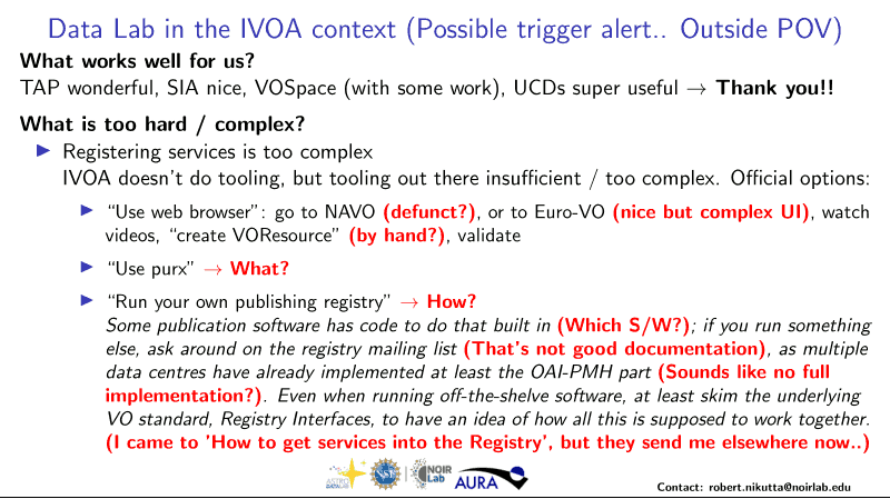
Now, I think I have to put up the defense that this was basically the abstract and there are more explanations further down the page, for instance on the “purx” that confused Robert so much[2]. More importantly, though: If you don't understand some VO documentation, it is rather likely that you are not the only one. You will not only help yourself but all these other people if you complain, ideally with suggestions on how to improve or perhaps concrete questions.
If it is not otherwise clear just who to complain to, use the mailing list of a working or interest group that sounds as if it might be responsible. I can't promise you we will improve matters, but knowing about a problem makes it a lot more likely someone will address it.
In Robert's concrete issue of a simple and straightforward OAI-PMH component, on the other hand, documentation is not enough. At least as long as I cannot convince the rest of the world that collaborating on DaCHS[3] is a much smarter move than everyone developing their own server software, there really should be such a thing, and I think I've charmed some of the self-implementors into collaborating in such an effort.
Traditionally, the last talk of an Interop is reserved for the chair of the Exec (the bosses of the national VO projects). They then reveal who the Exec has chosen as the future chairs and vice-chairs of the working and interest groups. I will not pretend that I was surprised: I will be vice chair of the solar system interest group in the next few years. And I already have a first project that came up during one of the many, many, many coffee break discussions of this Interop: finally start collecting planetary reference frames for the vocabulary of references frames. What a nice bridge from semantics to solar system!
| [1] | No, having to carry around and plug in and out some additional hardware is only marginally less annoying than the digit-copying 2FA schemes. |
| [2] | I will give you that my predilection for cute names is not always helpful, though. |
| [3] | DaCHS of course has an OAI-PMH interface built in, but that is so highly integrated with its metadata management and XML generation that pulling it out just is not worth it. |