Posts with the Tag ADQL:

  • ADQL Traps #1: NULL

    NULL is a difficult concept. Not only in SQL

    NULL is a difficult concept. Not only in SQL

    I recently got embarrassed by ADQL NULLs, i.e., the magic value indicating that a value in a given column is missing. And since that's a common source of errors when writing ADQL queries, I'll take this as a cue for a blog post.

    The concrete background is fairly technical and registry-ish; suffice it to say that some data providers who implemented interfaces conforming to some standard didn't properly say so in their registry records. Back in RegTAP 1.0 (that's the standard that says how a client like TOPCAT talks to the VO Registry), I decided to work around that by fudging the pattern for how to discover those interfaces so they'd still be found.

    In RegTAP 1.1, which is now under review by the VO community, I wanted to do away with that workaround. But would that break anything? This question translates to “are there vs:ParamHTTP interfaces that don't have a role attribute of std”. Whatever “ParamHTTP” and “role attribute” actually mean, just appreciate that it looks like it might translate into SQL like:

    select * from rr.interface
    where
      intf_type='vr:paramhttp'
      and not intf_role='std'
    

    I ran that query, rejoiced because it didn't return anything, removed the workarund from the standard, and then was shot down when I read Mark's mail (politely) saying I'm wrong and there are services still requiring the workaround. As usual: If a query returns what you expect, be double careful.

    What went wrong? Well, NULL semantics. You see, in SQL NULL is never equal to anything, not even itself (it's like NaN in IEEE floats in that: try n = float('nan');print(n==n) in Python and look again if you're cool about it). It's also not unequal. Don't take my word for it. Try:

    select * from tap_schema.schemas where NULL=NULL
    

    and:

    select * from tap_schema.schemas where NULL!=NULL
    

    – you'll get empty results in both cases.

    What does that mean for science queries? Well, whenever there's NULLs in columns (and the only safe assumption for now is that they may hide in there; we should probably add nun-null as a column property in the tap schema and in VODataService some day), you need to be careful in particular with inverted logic.

    Here's an example: Suppose you want to investigate NGC objects brighter than 10 mag in B in one bin in everything else in another. The ones brighter are simple:

    select count(*) from openngc.data where mag_b<10
    

    (try it on the TAP server at http://dc.g-vo.org/tap, it's 383 in the current release). It becomes difficult for “the rest”. If you write:

    select count(*) from openngc.data where not mag_b<10
    

    or, equivalently:

    select count(*) from openngc.data where mag_b>=10
    

    you'll get (for the current release) 10887. However, the whole catalogue has 13954 entries, so there's 13954-10887-383=2684 rows missing. Your “rest” has missed everything for which mag_b isn't given. Sure enough:

    select count(*) from openngc.data where mag_b is null
    

    (and this is the only good way to compare against null) gives 2684.

    The right way to say “anything for which mag_b is not smaller than 10” thus is:

    select count(*) from openngc.data
    where
      not mag_b<10
      or mag_b is null
    

    Morale: Unless you're sure there are no missing values (i.e., NULLs) in a column you're looking at, think about what these mean to your research (or other) question: Should these rows just vanish? Then you usually don't need to do anything and the SQL semantics magically do the right thing (which is why things are defined as they are). If, however, the corresponding rows would mean something to your question, you need to be explicit, and you must have some condition involving IS NULL or IS NOT NULL.

    The trouble, of course, is that just knowing this still isn't enough. You need to remember it in the right moment. Or you'll share my fate of suffering some public embarrassement.

  • APPLAUSE via Obscore

    A composite of two rather noisy photo plates

    Aladin showing some Bamberg Sky Patrol plates (see towards the end of the post for what this is and how I made it).

    At the Astroplate conference I blogged about recently, the people behind APPLAUSE gave a couple of talks about their Data Release 3. APPLAUSE is a fairly massive endeavour to make available data from some of the larger plate archives in Germany, and its DR3 even hit the non-Astronomy press last February.

    Already for previous APPLAUSE releases, I've wanted to bring this data (or rather, its metadata) to the VO, but it never quite happened, basically because there was always another little thing that turned out to be too tedious to work out via mail. However, working out things interactively is exactly what conferences are great for. So, the kind APPLAUSE folks (thanks, Taavi and Harry) and I used the Astroplate to map their database schema (“schema” is jargon for what boils down to the set of tables and columns with which they describe their data) to the much simpler (and, admittedly, less powerful) IVOA Obscore one.

    Sure, Obscore doesn't deal with multiple exposures (like when the target field and the north pole were exposed on one plate to help precision photometry), object-guided images, and all the other interesting techniques that astronomers applied in the pre-digital age; it also doesn't usefully cope with multiple scans of the same plate (for instance, to correct for imprecisions in the mechanics of flatbed scanners). APPLAUSE, of course, has to cope with them, since there are many reasons to preserve data of this kind.

    Obscore, on the other hand, is geared towards uniform discovery, where too funky datasets in all likelihood cause more harm than good. So, when we mapped APPLAUSE to Obscore, of the 101138 scans of 70276 plates that the full APPLAUSE holds in DR3, only 44000 plate scans made it into the Obscore table. The advantage: whatever can be sensibly mapped to Obscore can now be queried together with all the other data in the world that others have published through Obscore.

    You can immediately see the effect when you run the little python program doing the global discovery we gave in our plates tutorial. Here's what it prints now (values from pre-APPLAUSE-in-Obscore are in square brackets):

    Column t_exptime: 3460 values
      Min   12, Max 15300, Mean 890.24  [previous mean: 370.722]
    ---
    Column em_mean: 3801 values
      Min 1.8081e-09, Max 9.3e-07, Mean 6.40804e-07 [No change: Sigh!]
    ---
    Column t_mean: 4731 values
      Min 12564.5, Max 58126.3, Mean 49897.9 [previous mean: 51909.1]
    ---
    Column instrument_name: 4747 values
      Matches from , Petzval, [Max Wolf's residence in
      Heidelberg, Maerzgasse, Wolf's Doppelastrograph,
      Heidelberg Koenigstuhl (24), Wolf's
      Doppelastrograph,] AG-Astrograph, [Zeiss Triplet
      15 cm Potsdam-Telegrafenberg], Zeiss Triplet,
      Astrograph (four 10-cm Tessar f/6 cameras),
      [3.5m APO, ROSAT PSPCC, Heidelberg Koenigstuhl
      (24), Bruce Astrograph, Calar Alto (493),
      Schmidt], Grosser Refraktor, [ROSAT HRI,
      DK-1.54], Hamburger Schmidt-Spiegel,
      [DFOSC_FASU], ESO 1-metre Schmidt telescope,
      Great Schmidt Camera, Lippert-Astrograph, Ross-B
      3", [AZT 22], Astrograph (six 10-cm Tessar f/6
      cameras), 1m-Spiegelteleskop, [ROSAT PSPCB],
      Astrograph (ten 10-cm Tessar f/6 cameras), Zeiss
      Objective
    ---
    Column access_url: 4747 values [4067]
    

    So – for the fields selected in the tutorial, there are 15% more images in the global Obscore image pool now than there were before APPLAUSE, and their mean observation date went a bit farther into the past. I've not made any statistics, but I suspect for many other fields the gain is going to be much higher. For a strong effect, try some random region covered by the Bamberg Sky Patrol on the southern sky.

    But you have probably noticed the deep sigh in the annotations to the statistics above: Yes, we don't have the spectral band for the APPLAUSE data, which is why the stats on em_min doesn't change. As a matter of fact, from the Obscore data you can't even guess whether a plate is “more red” or “rather blue”, as Obscore doesn't have an (agreed-upon) field for “qualititive bandpass indicator”.

    For some other data collections, we did map known emulsion/filter combinations to rough bandpasses (e.g., the Palomar-Leiden Trojan Survey, which only had a few of them). For APPLAUSE, there are 435 combinations of filter and emulsion (that's a VOTable link that you can paste into TOPCAT's load button in order to have a look at the table). Granted, quite a few of these pairs are (more or less) spurious because of inconsistent spelling. But we still gave up on researching the bandpasses even before we started.

    If you're a photographic plate buff: You could help us and posteriority a lot if you could go through this list and at least for some combinations tell us what, roughly, the lower and upper limits of the corresponding bandpasses might have been (what DaCHS already knows, plate-relevant data near the bottom of the file). As usual, send mail to gavo@ari.uni-heidelberg.de if you have anything to contribute.

    Finally, here's the brief explanation of the image for this article: Well, I wanted to find some Bamberg Sky Patrol images for a single field to play with. I knew they were primarily located in the South, and were made using Tessar cameras. So, I ran:

    SELECT t_min, access_url, s_region
    FROM ivoa.obscore
    WHERE instrument_name like '%Tessar%'
    AND 1=CONTAINS(POINT(345, -38), s_region)
    

    on GAVO's TAP service. Since Aladin 10, you can do that from within the program (although some versions will reject this query because they mistakenly believe the ADQL is bad. Query through TOPCAT and send the result over to Aladin if that bites you). Incidentally, when there are s_region values in Obscore tables, it's a good idea to use them as I do here, as it's quite a bit more likely that this query will use indices than some condition on s_ra and s_dec. But then not all services fill s_region properly, so for all-VO queries you will probably want to make do with s_ra and s_dec.

    From that result I first made the inset bar graph in the article image to show the temporal distribution of the Patrol plates. And then I grabbed two (rather randomly selected) plates and had Aladin produce a red-blue composite of them. Whatever is really red or really blue in that image may correspond to a transient event. Or, as certainly the case with that little hair (or whatever) that shines out in blue, it may not.

  • Find Outliers using ADQL and TAP

    Annie Cannon's notebook and a plot

    Two pages from Annie Cannon's notebooks[1], and a histogram of the basic BP-RP color distribution in the HD catalogue (blue) and the distribution of the outliers (red). For more of Annie Cannon's notebooks, search on ADS.

    The other day I gave one of my improvised live demos (“What, roughly, are you working on?”) and I ended up needing to translate identifiers from the Henry Draper Catalogue to modern positions. Quickly typing “Henry Draper” into TOPCAT's TAP search window didn't yield anything useful (some resources only using the HD, and a TAP service that didn't support uploads – hmpf).

    Now, had I tried the somewhat more thorough WIRR Registry interface, I'd have noted the HD catalogue at VizieR and in particular Fabricius' et al's HD-Tycho 2 match (explaining why they didn't show up in TOPCAT is a longer story; we're working on it). But alas, I didn't, and so I set out to produce a catalogue matching HD and Gaia DR2, easily findable from within TOPCAT's TAP client. Well, it's here in the form of the hdgaia.main table in our data center.

    Considering the nontrivial data discovery and some yak shaving I had to do to get from HD identifiers to Gaia DR2 ones, it was perhaps not as futile an exercise as I had thought now and then during the preparation of the thing. And it gives me the chance to show a nice ADQL technique to locate outliers.

    In this case, one might ask: Which objects might Annie Cannon and colleagues have misclassified? Or perhaps the objects have changed their spectrum between the time Cannon's photographic plates have been taken and Gaia observed them? Whatever it is: We'll have to figure out where there are unusual BP-RPs given the spectral type from HD.

    To figure this out, we'll first have to determine what's “usual”. If you've worked through our ADQL course, you know what to expect: grouping. So, to get a table of average colours by spectral type, you'd say (all queries executable on the TAP service at http://dc.g-vo.org/tap):

    select spectral,
      avg(phot_bp_mean_mag-phot_rp_mean_mag) as col,
      count(*) as ct
    from hdgaia.main
    join gaia.dr2light
    using (source_id)
    group by spectral
    

    – apart from the join that's needed here because we want to pull photometry from gaia, that's standard fare. And that join is the selling point of this catalog, so I won't apologise for using it already in the first query.

    The next question is how strict we want to be before we say something that doesn't have the expected colour is unusual. While these days you can rather easily use actual distributions, at least for an initial analysis just assuming a Gaussian and estimating its FWHM as the standard deviation works pretty well if your data isn't excessively nasty. Regrettably, there is no aggregate function STDDEV in ADQL (you could still ask for it: head over to the DAL mailing list before ADQL 2.1 is a done deal!). However, you may remember that Var(X)=E(X2)-E(X)2, that the average is an estimator for the expectation, and that the standard deviation is actually an estimator for the square root of the variance. And that these estimators will work like a charm if you're actually dealing with Gaussian data.

    So, let's use that to compute our standard deviations. While we are at it, throw out everything that's not a star[2], and ensure that our groups have enough members to make our estimates non-ridiculous; that last bit is done through a HAVING clause that essentially works like a WHERE, just for entire GROUPs:

    select spectral,
      avg(phot_bp_mean_mag-phot_rp_mean_mag) as col,
      sqrt(avg(power(phot_bp_mean_mag-phot_rp_mean_mag, 2))-
        power(avg(phot_bp_mean_mag-phot_rp_mean_mag), 2)) as sig_col,
      count(*) as ct
    from hdgaia.main
    join gaia.dr2light
      using (source_id)
    where m_v<18
    group by spectral
    having count(*)>10
    

    This may look a bit scary, but if you read it line by line, I'd argue it's no worse than our harmless first GROUP BY query.

    From here, the step to determine the outliers isn't big any more. What the query I've just written produces is a mapping from spectral type to the means and scales (“µ,σ” in the rotten jargon of astronomy) of the Gaussians for the colors of the stars having that spectral type. So, all we need to do is join that information by spectral type to the original table and then see which actual colors are further off than, say, three sigma. This is a nice application of the common table expressions I've tried to sell you in the post on ADQL 2.1; our determine-what's-usual query from above stays nicely separated from the (largely trivial) rest:

    with standards as (select spectral,
      avg(phot_bp_mean_mag-phot_rp_mean_mag) as col,
      sqrt(avg(power(phot_bp_mean_mag-phot_rp_mean_mag, 2))-
        power(avg(phot_bp_mean_mag-phot_rp_mean_mag), 2)) as sig_col,
      count(*) as ct
      from hdgaia.main
      join gaia.dr2light
      using (source_id)
      where m_v<18
      group by spectral
      having count(*)>10)
    select *
    from hdgaia.main
    join standards
    using (spectral)
    join gaia.dr2light using (source_id)
    where
      abs(phot_bp_mean_mag-phot_rp_mean_mag-col)>3*sig_col
      and m_v<18
    

    – and that's a fairly general pattern for doing an initial outlier analysis on the the remote side. For HD, this takes a few seconds and yields 2722 rows (at least until we also push HDE into the table). That means you can keep 99% of the rows (the boring ones) on the server and can just pull the ones that could be interesting. These 99% savings aren't terribly much with a catalogue like the HD that's small by today's standards. For large catalogs, it's the difference between a download of a couple of minutes and pulling data for a day while frantically freeing disk space.

    By the way, that there's only 2.7e3 outliers among 2.25e5 objects, while Annie Cannon, Williamina Fleming, Antonia Maury, Edward Pickering, and the rest of the crew not only had to come up with the spectral classification while working on the catalogue but also had to classify all these objects manually. This is an amazing feat even if all of those rows actually were misclassifications (which they certainly aren't) – the machine classifiers of today would be proud to only get 1% wrong.

    The inset in the facsimile of Annie Cannons notebooks above shows how the outliers are distributed in color space relative to the full catalogue, where the basic catalogue is in blue and the outliers (scaled by 70) in red. Wouldn't it make a nice little side project to figure out the reason for the outlier clump on the red side of the histogram?

    [1]The notebook pages are from a notebook Annie Cannon used in 1929. The material was kindly provided by Project PHAEDRA at the John G. Wolbach Library, Harvard College Observatory.
    [2]I'll not hide that I was severely tempted to undo the mapping of object classes to – for HD – unrealistic magnitudes (20 .. 50) but then left the HD as it came from ADC; I still doubt that decision was well taken, and sure enough, the example query above already has insane constraints on m_v reflecting that encoding. From today's position, of course there should have been an extra column or, better yet, a different catalogue for nonstellar objects. Ah well. It's always hard to break unhealty patterns.
  • Deredden using TAP

    An animated color-magnitude diagram

    Raw and dereddened CMD for a region in Cygnus.

    Today I published a nice new set of tables on our TAP service: The Bayestar17 3D dust map derived from Pan-STARRS 1 by Greg Green et al. I mention in passing that this was made particularly enjoyable because Greg and friends put an explicit license on their data (in this case, CC-BY-SA).

    This dust map is probably a fascinating resource by itself, but the really nifty thing is that you can use it to correct all kinds of photometric data for extinction – at least to some extent. On the Bayestar web page, the authors give some examples for usage – and with our new service, you can use TAP as well to correct photometry for extinction.

    To see how, first have a look at the table metadata for the prdust.map_union table; this is what casual users probably should look at. More specifically, at the coverage, best_fit, and grdiagnostic columns.

    coverage here is an interval of 10-healpixes. It has to be an interval because the orginal data comes on wildly different levels; depending on the density of stars, sometimes it takes the area of a 6-healpix (about a square degree) to get enough signal, whereas in the galactic plane a 10-healpix (a thousandth of a square degree) already has enough stars. To make the whole thing conveniently queriable without exploding a 6-healpix row into 1000 identical rows, larger healpixes translate into intervals of 10-helpixes. Don't panic, though, I'll show how to conveniently query this below.

    best_fit and grdiagnostic are arrays (remember the light cuves in Gaia DR2?). In bins of 0.5 in distance modulus (which is, in case you feel a bit uncertain as to the algebraic signs, 5 log10(dist)-5 for a distance in parsec), starting with a distance modulus of 4 and ending with 19. This means that for a distance modulus of 4.2 you should check the array index 0, whereas 4.3 already would be covered by array index 1. With this, best_fit[ind] gives E(B-V) = (B-V) - (B-V)0 in the direction of coverage in a distance modulus bin of 2*ind+4. For each best_fit[ind], grdiagnostic[ind] contains a quality measure for that value. You probably shouldn't touch the E(B-V) if that measure is larger than 1.2.

    So, how does one use this?

    To try things, let's pull some Gaia data with distances; in order to have interesting extinctions, I'm using a patch in Cygnus (RA 288.5, Dec 2.3). If you live on the northern hemisphere and step out tonight, you could see dust clouds there with the naked eye (provided electricity fails all around, that is). Full disclosure: I tried the Coal Sack first but after checking the coverage of the dataset – which essentially is the sky north of -30 degrees – I noticed that wouldn't fly. But stories like these are one reason why I'm making such a fuss about having standard STC coverage representations.

    We want distances, and to dodge all the intricacies involved when naively turning parallaxes to distances discussed at length in a paper by Xavier Luri et al (and elsewhere), I'm using precomputed distances from Bailer-Jones et al. (2018AJ....156...58B); you'll find them on the "ARI Gaia" service; in TOPCAT's TAP dialog simply search for “Gaia” – that'll give you the GAVO DC TAP search, too, and that we'll need in a second.

    The pre-computed distances are in the gaiadr2_complements.geometric_distance table, which can be joined to the main Gaia object catalog using the source_id column. So, here's a query to produce a little photometric catalog around our spot in Cygnus (we're discarding objects with excessive parallax errors while we're at it):

    SELECT
    r_est, 5*log10(r_est)-5 as dist_mod,
    phot_g_mean_mag, phot_bp_mean_mag, phot_rp_mean_mag,
    ra, dec
    FROM
    gaiadr2.gaia_source
    JOIN gaiadr2_complements.geometric_distance
    USING (source_id)
    WHERE
    parallax_over_error>1
    AND 1=CONTAINS(POINT('ICRS', ra, dec), CIRCLE('ICRS', 288.5, 2.3, 0.5 ))
    

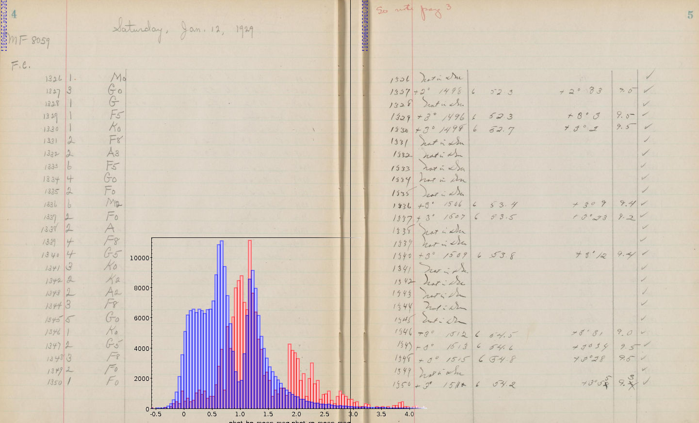
    The color-magnitude diagram resulting from this is the red point cloud in the animated GIF at the top. To reproduce it, just plot phot_bp_mean_mag-phot_rp_mean_mag against phot_g_mean_mag-dist_mod (and invert the y axis).

    De-reddening this needs a few minor technicalities. The most important one is how to match against the odd intervals of healpixes in the prdust.map_union table. A secondary one is that we have only pulled equatorial coordinates, and the healpixes in prdust are in galactic coordinates.

    Computing the healpix requires the ivo_healpix_index ADQL user defined function (UDF) that you may have met before, and since we have to go from ICRS to Galactic it requires a fairly new UDF I've recently defined to finally get the discussion on having a “standard library” of astrometric functions in ADQL going: gavo_transform. Here's how to get a 10-healpix as required for map_union from ra and dec:

    CAST(ivo_healpix_index(10,
      gavo_transform('ICRS', 'GALACTIC', POINT(ra, dec))) AS INTEGER)
    

    The CAST call is a pure technicality – ivo_healpix_index returns a 64-bit integer, which I can't use in my interval logic.

    The comparison against the intervals you could do yourself, but as argued in Registry-STC article this is one of the trivial things that are easy to get wrong. So, let's use the ivo_interval_overlaps UDF; it goes in the join condition to properly match prdust healpixes to catalog positions. Then our total query – that, I hope, should be reasonably easy to adapt to similar problems – is:

    WITH sources AS (
      SELECT phot_g_mean_mag,
        phot_bp_mean_mag,
        phot_rp_mean_mag,
        dist_mod,
        CAST(ivo_healpix_index(10,
          gavo_transform('ICRS', 'GALACTIC', POINT(ra, dec))) AS INTEGER) AS hpx,
        ROUND((dist_mod-4)*2)+1 AS dist_mod_bin
      FROM TAP_UPLOAD.T1)
    
    SELECT
      phot_bp_mean_mag-phot_rp_mean_mag-dust.best_fit[dist_mod_bin] AS color,
      phot_g_mean_mag-dist_mod+
        dust.best_fit[dist_mod_bin]*3.384 AS abs_mag,
      dust.grdiagnostic[dist_mod_bin] as qual
    FROM sources
    JOIN prdust.map_union AS dust
    ON (1=ivo_interval_has(hpx, coverage))
    

    (If you're following along: you have to switch to the GAVO DC TAP to run this, and you will probably have to change the index after TAP_UPLOAD).

    Ok, in the photometry department there's a bit of cheating going on here – I'm correcting Gaia B-R with B-V, and I'm using the factor for Johnson V to estimate the extinction in Gaia G (if you're curious where that comes from: See the footnote on best_fit and the MC extinction service docs should get you started), so this is far from physically correct. But, as you can see from the green cloud in the plot above, it already helps a bit. And if you find out better factors, by all means let me know so I can add an update... right here:

    Update (2018-09-11): The original data creator, Gregory Green points out that the thing with having a better factor for Gaia G isn't that simple, because, as he says “Gaia G is very broad, [and] the extinction coefficients are much more dependent on stellar type, and extinction is also more nonlinear with dust column (extinction is only linear with dust column and independent of stellar type for an infinitely narrow passband)”. So – when de-reddening, prefer narrow passbands. But whether narrow or wide: TAP helps you.

  • DaCHS 1.2 is out

    Today, I have released DaCHS 1.2 – somewhat belatedly perhaps, because I managed to break my collarbone, but here it is. If you've been following this blog, you already know about the headline news: the dachs start command, ADQL 2.1, and early support for STC in the registry.

    If you're not yet on DaCHS 1.1, please have a quick look at the corresponding release article. While the upgrade itself should work fine in one go even from older versions, the release notes of course apply cumulatively, and you may still have to do the dist-upgrade to 1.1.

    As usual, the generic upgrading instructions are available in the operator's guide (in short: do a dachs val ALL; apt update; apt upgrade). Since I've still encountered DaCHS installations with wrong sources.lists last April: Note again that our repository names have changed in August 2016 – we now have release and beta rather than Debian release names. So, make sure you have something like:

    deb http://vo.ari.uni-heidelberg.de/debian release main
    

    in your /etc/apt/sources.list, not something containing “stable” or the like.

    That said, here's the commented changes for 1.2:

    • New dachs start command to produce structured templates for certain service types. See Horror Vacui Begone on this blog for the full story.
    • Support for ADQL 2.1 (actually, its current proposed recommendation), including almost all of the optional parts (see Speak out on ADQL 2.1 on this blog). While not strictly necessary, it's a good idea to run dachs imp //adql after the upgrade; this will give you some nice new UDFs, in particular gavo_histogram.
    • New coverage element (with updaters) to build and declare the space-time-spectral coverage of a resource. It would be great if you could add coverage elements to your resources where it makes sense and re-publish them. This blog post tells you how to do it (you'll have to scroll down a bit).
    • There is now odbcGrammar to feed an import from another database. Essentially, you put an ODBC connection string into a file, point your sources element there, and you'll get one rawdict per tuple in a foreign database table. This might be a nice way to publish moderate-size non-postgres tables via DaCHS.
    • You can now declare associated datalink services for tables using the _associatedDatalinkSvc meta item. In particular, if you had a datalink property on SSAP services, you should migrate at some point. One advantage: Users will get the datalinks even when querying the tables through TAP. See “Integrating Datalink Services” in the reference documentation for the full story.
    • We now force matplotlib to read its configuration from /var/gavo/etc/matplotlibrc; to get a default, just run dachs init again. This is mainly to avoid uncontrolled imports of matplotlibrcs when DaCHS is run under a uid that does other things now and then.
    • DaCHS now supports VOSI 1.1; in particular, DaCHS now understands the detail hints and has per-table endpoints, so clients like TOPCAT could avoid reading the full table metadata in one go. Realistically, at least TOPCAT doesn't yet, so this is perhaps less cool than it may sound.
    • The indices generated by the ssa mixins are now a bit more sensible considering typical query modes. You probably want to run dachs imp -I on the RDs for your ssap data collections when convenient. If you have larger spectral collections, chances are many queries will be a lot faster.
    • ssapCore no longer wantonly adds preview columns. If you have previews with spectra, you probably want to add <property name="previews">auto</property> to your ssapCores. If you don't, the preview column will not be added to SSA responses (right now, few clients evaluate it, but that will hopefully change in the future).
    • You can now add a statisticsTarget property to columns; you will want this on largish tables with non-uniformly distributed values to aid the query planner; something like <property key=" statisticsTarget">10000</property> within the corresponding column element can go a long way to improve query planning (you need to run gavo imp -m on the RD after the change).
    • DaCHS's log now by default does not contain IP addresses, user agents, and referrers any more, which should mostly keep you from processing personal data and thus from having to muck around with the EU GDPR. To get back the previous behaviour, set [web]logFormat in /etc/gavo.rc to combined.
    • I fixed some utypes for obscore 1.1. These utypes are useless, so there's nothing you have to do. But then stilts taplint complains about them, and so you may want to run dachs imp -m //obscore.
    • As usual, there are many minor bug fixes and improvements (e.g., memmapping FITSes for cutout again, delimited table references in ADQL, new-style tutorial resource records, correct obscore standardId, much saner nD-arrays in VOTables).

    Well – enjoy the release, and if something goes wrong with it, be sure to let us know, preferably on the DaCHS-suppport mailing list.

« Page 5 / 7 »