Histograms and Hidden Open Clusters
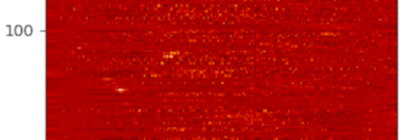
Colour-coded histograms for distances of stars in the direction of some NGC open clusters -- one cluster per line, so you're looking a a couple of Gigabytes of data here. If you want this a bit more precise: Read the article and generate your own image.
I have spent a bit of time last week polishing up what will (hopefully) be the definitive source of common ADQL User Defined Functions (UDFs) for IVOA review. What's a UDF, you ask? Well, it is an extension to ADQL where service operators can invent new functionality. If you have been following this blog for a while, you will probably remember the ivo_healpix_index function from our dereddening exercise (and some earlier postings): That was an UDF, too.
This polishing work reminded me of a UDF I've wanted to blog about for a quite a while, available in DaCHS (and thus on our Heidelberg Data Center) since mid-2018: gavo_histogram. This, I claim, is a powerful tool for analyses over large amounts of data with rather moderate local means.
For instance, consider this classic paper on the nature of NGC 2451: What if you were to look for more cases like this, i.e., (indulging in a bit of poetic liberty) open clusters hidden “behind” other open clusters?
Somewhat more technically this would mean figuring out whether there are “interesting” patterns in the distance and proper motion histograms towards known open clusters. Now, retrieving the dozens of millions of stars that, say, Gaia, has in the direction of open clusters to just build histograms – making each row count for a lot less than one bit – simply is wasteful. This kind of counting and summing is much better done server-side.
On the other hand, SQL's usual histogram maker, GROUP BY, is a bit unwieldy here, because you have lots of clusters, and you will not see anything if you munge all the histograms together. You could, of course, create a bin index from the distance and then group by this bin and the object name, somewhat like ...ROUND(r_est/20) as bin GROUP by name, bin – but that takes quite a bit of mangling before it can conveniently be used, in particular when you take independent distributions over multiple variables (“naive Bayesian”; but then it's the way to go if you want to capture dependencies between the variables).
So, gavo_histogram to the rescue. Here's what the server-provided documentation has to say (if you use TOPCAT, you will find this in the ”Service” tab in the TAP windows' ”Use Service” tab):
gavo_histogram(val REAL, lower REAL, upper REAL, nbins INTEGER) -> INTEGER[]

The aggregate function returns a histogram of val with
nbins+2 elements. Assuming 0-based arrays, result[0] contains
the number of underflows (i.e., val<lower), result[nbins+1]
the number of overflows. Elements 1..nbins are the counts in
nbins bins of width (upper-lower)/nbins. Clients will have to
convert back to physical units using some external communication,
there currently is no (meta-) data as to what lower and upper was in
the TAP response.
This may sound a bit complicated, but the gist really is: type gavo_histogram(r_est, 0, 2000, 20) as hist, and you will get back an array with 20 bins, roughly 0..100, 100..200, and so on, and two extra bins for under- and overflows.
Let's try this for our open cluster example. The obvious starting point is selecting the candidate clusters; we are only interested in famous clusters, so we take them from the NGC (if that's too boring for you: with TAP uploads you could take the clusters from Simbad, too), which conveniently sits in my data center as openngc.data:
select name, raj2000, dej2000, maj_ax_deg
from openngc.data
where obj_type='OCl'
Then, we need to add the stars in their rough directions. That's a classic crossmatch, and of course these days we use Gaia as the star catalogue:
select name, source_id
from openngc.data
join gaia.dr2light
on (
  1=contains(
    point(ra,dec),
    circle(raj2000, dej2000, maj_ax_deg)))
where obj_type='OCl')
This is now a table of cluster names and Gaia source ids of the candidate stars. To add distances, you could fiddle around with Gaia parallaxes, but because there is a 1/x involved deriving distances, the error model is complicated, and it is much easier and safer to adopt Bailer-Jones et al's pre-computed distances and join them in through source_id.
And that distance estimation, r_est, is exactly what we want to take our histograms over – which means we have to group by name and use gavo_histogram as an aggregate function:
with ocl as (
  select name, raj2000, dej2000, maj_ax_deg, source_id
  from openngc.data
  join gaia.dr2light
  on (
    1=contains(
      point(ra,dec),
      circle(raj2000, dej2000, maj_ax_deg)))
  where obj_type='OCl')

select
  name,
  gavo_histogram(r_est, 0, 4000, 200) as hist
from
  gdr2dist.main
  join ocl
  using (source_id)
where r_est!='NaN'
group by name
That's it! This query will give you (admittedly somewhat raw, since we're ignoring the confidence intervals) histograms of the distances of stars in the direction of all NGC open clusters. Of course, it will run a while, as many millions of stars are processed, but TAP async mode easily takes care of that.
Oh, one odd thing is left to discuss (ignore this paragraph if you don't know what I'm talking about): r_est!='NaN'. That's not quite ADQL but happens to do the isnan of normal programming languages at least when the backend is Postgres: It is true if computations failed and there is an actual NaN in the column. This is uncommon in SQL databases, and normal NULLs wouldn't hurt gavo_histogram. In our distance table, some NaNs slipped through, and they would poison our histograms. So, ADQL wizards probably should know that this is what you do for isnan, and that the usual isnan test val!=val doesn't work in SQL (or at least not with Postgres).
So, fire up your TOPCAT and run this on the TAP server http://dc.g-vo.org/tap.
You will get a table with 618 (or so) histograms. At this point, TOPCAT can't do a lot with them. So, let's emigrate to pyVO and save this table in a file ocl.vot
My visualisation proposition would be: Let's substract a “background” from the histograms (I'm using splines to model that background) and then plot them row by row; multi-peaked rows in the resulting image would be suspicious.
This is exactly what the programme below does, and the image for this article is a cutout of what the code produces. Set GALLERY = True to see how the histograms and background fits look like (hit 'q' to get to the next one).
In the resulting image, any two yellow dots in one line are at least suspicious; I've spotted a few, but they are so consipicuous that others must have noticed. Or have they? If you'd like to check a few of them out, feel free to let me know – I think I have a few ideas how to pull some VO tricks to see if these things are real – and if they've been spotted before.
So, here's the yellow spot programme:
from astropy.table import Table
import matplotlib.pyplot as plt
import numpy
from scipy.interpolate import UnivariateSpline

GALLERY = False

def substract_background(arr):
    x = range(len(arr))
    mean = sum(arr)/len(arr)
    arr = arr/mean
    background = UnivariateSpline(x, arr, s=100)
    cleaned = arr-background(x)

    if GALLERY:
        plt.plot(x, arr)
        plt.plot(x, background(x))
        plt.show()

    return cleaned


def main():
    tab = Table.read("ocl.vot")
    hist = numpy.array([substract_background(r["hist"][1:-1])
      for r in tab])
    plt.matshow(hist, cmap='gist_heat')
    plt.show()


if __name__=="__main__":
    main()

![[RSS]](../theme/image/rss.png)

