![[RSS]](../theme/image/rss.png)
Spectral Units in ADQL
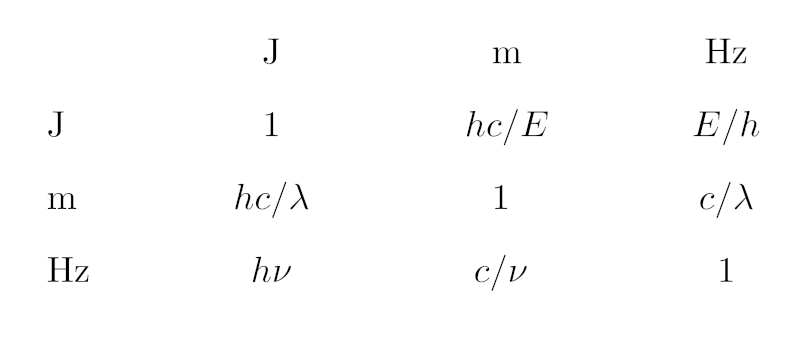
In case you find the piece of Python given below too hard to read: It's just this table of conversion expressions between the different SI units we are dealing with here.
Astronomers these days work all along the electromagnetic spectrum (and beyond, of course). Depending on where they observe, they will have very different instrumentation, and hence some see their messengers very naturally as waves, others quite as naturally as particles, others just as electrons flowing out of a CCD that is sitting behind a filter.
In consequence, when people say where in the spectrum they are, they use very different notions. A radio astronomer will say “I'm observing at 21 cm” or “at 50 GHz“. There's an entire field named after a wavelength, “submillimeter“, and blueward of that people give their bands in micrometers. Optical astronomers can't be cured of their Ångström habit. Going still more high-energy, after an island of nanometers in the UV you end up in the realm of keV in X-ray, and then MeV, GeV, TeV and even EeV.
However, there is just one VO (or at least that's where we want to go). Historically, the VO has had a slant towards optical astronomy, which gives us the legacy of having wavelengths in far too many places, including Obscore. Retrospectively, this was an unfortunate choice not only because it makes us look optical bigots, but in particular because in contrast to energy and, by ν = E/h, frequency, messenger wavelength depends on the medium you work in, and I shudder to think how many wavelengths in my data center actually are air wavelengths rather than vacuum wavelengths. Also, as you go beyond photons, energy really is the only thing that reasonably characterises all messengers alike (well, even that still isn't quite settled for gravitational waves as long as we're not done with a quantum theory of gravitation).
Well – the wavelength milk is spilled. Still, the VO has been boldly expanding its reach beyond the optical and infrared windows (recently, with neutrinos and gravitational waves, not to mention EPN-TAP's in-situ measurements in the solar system, even beyond the electromagnetic spectrum). Which means we will have to accomodate the various customs regarding spectral units described above. Where there are “thick” user interfaces, these can care about that. For instance, my datalink XSLT and javascript lets people constrain spectral cutouts (along BAND) in a variety of units (Example).
But what if the UI is as shallow as it is in ADQL, where you deal with whatever is in the underlying database tables? This has come up again at last week's EuroVO Technology Forum in virtual Strasbourg in the context of making Obscore more attractive to radio astronomers. And thus I've sat down and taught DaCHS a new user defined function to address just that.
Up front: When you read this in 2022 or beyond and everything has panned out, the function might be called ivo_specconv already, and perhaps the arguments have changed slightly. I hope I'll remember to update this post accordingly. If not, please poke me to do so.
The function I'm proposing is, mainly, gavo_specconv(expr, target_unit). All it does is convert the SQL expression expr to the (spectral) target_unit if it knows how to do that (i.e., if the expression's unit and the target unit are spectral units properly written in VOUnit) and raise an error otherwise.
So, you can now post:
SELECT TOP 5 gavo_specconv(em_min, 'GHz') AS nu
FROM ivoa.obscore
WHERE gavo_specconv((em_min+em_max)/2, 'GHz')
    BETWEEN 1 AND 2
  AND obs_collection='VLBA LH sources'
to the TAP service at http://dc.g-vo.org/tap. You will get your result in GHz, and you write your constraint in GHz, too. Oh, and see below on the ugly constraint on obs_collection.
Similarly, an X-ray astronomer would say, perhaps:
SELECT TOP 5 access_url, gavo_specconv(em_min, 'keV') AS energy
FROM ivoa.obscore
WHERE gavo_specconv((em_min+em_max)/2, 'keV')
  BETWEEN 0.5 AND 2
  AND obs_collection='RASS'
This works because the ADQL translator can figure out the unit of its first argument. But, perhaps regrettably, ADQL has no notion of literals with units, and so there is no way to meaningfully say the equivalent of gavo_specconv(656, 'Hz') to get Hα in Hz, and you will receive a (hopefully helpful) error message if you try that.
However, this functionality is highly desirable not the least because the queries above are fairly inefficient. That's why I added the funny constraints on the collection: without them, the queries will take perhaps half a minute and thus require async operation on my box.
The (fundamental) reason for that is that postgres is not smart enough to work out it could be using an index on em_min and em_max if it sees something like nu between 3e8/em_min and 3e7/em_max by re-writing the constraint into 3e8/nu between em_min and em_max (and think really hard about whether this is equivalent in the presence of NULLs). To be sure, I will not teach that to my translation layer either. Not using indexes, however, is a recipe for slow queries when the obscore table you query has about 85 million rows (hi there in 2050: yes, that was a sizable table in our day).
To let users fix what's too hard for postgres (or, for that matter, the translation engine when it cannot figure out units), there is a second form of gavo_specconv that takes a third argument: gavo_specconv(expr, unit_of_expr, target_unit). With that, you can write queries like:
SELECT TOP 5 gavo_specconv(em_min, 'Angstrom') AS nu
FROM ivoa.obscore
WHERE gavo_specconv(5000, 'Angstrom', 'm')
  BETWEEN em_min AND em_max
and hope the planner will use indexes. Full disclosure: Right now, I don't have indexes on the spectral limits of all tables contributing to my obscore table, so this particular query only looks fast because it's easy to find five datasets covering 500 nm – but that's an oversight I'll fix soon.
Of course, to make this functionality useful in practice, it needs to be available on all obscore services (say) – only then can people run all-VO obscore searches without the optical bias. The next step (before Bambi-eyeing the TAP implementors) therefore would be to get it into the catalogue of ADQL user defined functions.
For this, one would need to specify a bit more carefully what units must minimally be supported. In DaCHS, I have built this on a full implementation of VOUnits, which means you can query using attoparsecs of wavelength and get your result in dekaerg (which is a microjoule: 1 daerg = 1 uJ in VOUnits – don't you just love this?):
SELECT gavo_specconv(
  (spectral_start+spectral_end)/2, 'daerg')
  AS energy
FROM rr.stc_spectral
WHERE gavo_specconv(0.0002, 'apc', 'J')
  BETWEEN spectral_start AND spectral_end
(stop computing: an attoparsec is about 3 cm). This, incidentally, queries the draft RegTAP extension for the VODataService 1.2 coverage in space, time, and spectrum, which is another reason I'm proposing this function: I'm not quite sure how well my rationale that using Joules of energy is equally inconvenient for all communities will be generally received. The real rationale – that Joule is the SI unit for energy – I don't dare bring forward in the first place.
Playing with wavelengths in AU (you can do that, too; note, though, that VOUnit forbids prefixes on AU, so don't even try mAU) is perhaps entertaining in a slightly twisted way, but admittedly poses a bit of a challenge in implementation when one does not have full VOUnits available. I'm currently thinking that m, nm, Angstrom, MHz, GHz, keV and MeV (ach! No Joule! But no erg, either!) plus whatever spectral units are in use in the local tables would about cover our use cases. But I'd be curious what other people think.
Since I found the implementation of this a bit more challenging than I had at first expected, let me say a few words on how the underlying code works; I guess you can stop reading here unless you are planning to implement something like this.
The fundamental trouble is that spectral conversions are non-linear. That means that what I do for ADQL's IN_UNIT – just compute a conversion factor and then multiply that to whatever expression is in its first argument – will not work. Instead, one has to write a new expression. And building these expressions becomes involved because there are thousands of possible combinations of input and output units.
What I ended up doing is adopting standard (i.e., SI) units for energy (J), wavelength (m), and frequency (Hz) as common bases, and then first convert the source and target units to the applicable standard unit. This entails trying to convert each input unit to each standard unit until a conversion actually works, which in DaCHS' Python looks like this:
def toStdUnit(fromUnit):
    for stdUnit in ["J", "Hz", "m"]:
        try:
             factor = base.computeConversionFactor(
                 fromUnit, stdUnit)
        except base.IncompatibleUnits:
            continue
        return stdUnit, factor

    raise common.UfuncError(
        f"specconv: {fromUnit} is not a spectral unit understood here")
The VOUnits code is hidden away in base.computeConversionFactor, which raises an IncompatibleUnits when a conversion is impossible; hence, in the end, as a by-product this function also determines what kind of spectral value (energy, frequency, or wavelength) I am dealing with.
That accomplished, all I need to do is look up the conversions between the basic units, which can be done in a single dictionary mapping pairs of standard units to the conversion expression templates. I have not tried to make these templates particularly pretty, but if you squint, you can still, I hope, figure out this is actually what the opening image shows:
SPEC_CONVERSION = {
    ("J", "m"): "h*c/(({expr})*{f})",
    ("J", "Hz"): "({expr})*{f}/h",
    ("J", "J"): "({expr})*{f}",
    ("Hz", "m"): "c/({expr})/{f}",
    ("Hz", "Hz"): "{f}*({expr})",
    ("Hz", "J"): "h*{f}*({expr})",
    ("m", "m"): "{f}*({expr})",
    ("m", "Hz"): "c/({expr})/{f}",
    ("m", "J"): "h*c/({expr})/{f}",}
expr is (conceptually) replaced by the first argument of the UDF, and f is the conversion factor between the input unit and the unit expr is in. Note that thankfully, no additive operators are involved and thus all this is numerically well-conditioned. Hence, I can afford not attempting to simplify any of the expressions involved.
The rest is essentially book-keeping, where I'm using the ADQL parser to turn the expression into a tree fragment and then fiddling in the tree fragment for expr into that. The result then replaces the UDF function call in the syntax tree. You can review all this in context in DaCHS' ufunctions.py, starting at the definition of toStdUnit.
Sure: this is no Turing award material. But perhaps these notes are useful when people want to put this kind of thing into their ADQL engines. Which I'd consider a Really Good Thing™.