2022-10-07
Markus Demleitner
When I showed off my rendering of the Gaia DR 3 XP spectra a month ago,
I promised I would later show how my proposal for a Vector extension to
ADQL would enable quite a bit of interesting functionality on that
table. Let me make good on this promise with a little project to find
candidates for Wolf-Rayet stars, more specifically, WC stars. I give
you that's a bit cheap because they have very distinctive spectral
features, but then this is supposed to be a quick educational posting,
not a science paper.
Before I start, I probably should stress that in this context I am using
the word “vector” like a computer guy would. We are talking about
one-dimensional arrays here, not about the vectors the mathematicians
have given us (as in “elements of vector spaces“).
Getting Spectra for Wolf-Rayet Stars
Let us first produce a list of Wolf-Rayet stars (of any denomination)
using SIMBAD. So, start TOPCAT, open the TAP dialog and find the SIMBAD
TAP server. Run:
SELECT main_id, ra, dec
FROM basic
WHERE otype='WR*'
there. In the next step, we will need the Gaia DR3
source_ids for these objects, and so it would be nice to pull them
immediately from Simbad; you could in principle do that by running:
SELECT main_id, ra, dec, id
FROM basic
  JOIN ident
  ON (oid=oidref)
WHERE otype='WR*'
  AND id LIKE 'Gaia DR3%'
– but for one, fiddling out the actual source_ids from the strings you
get in the id column is a bit tedious, and then quite a few of these
objects don't have Gaia ids yet: The first query returns 1548 at the
moment, the second 696.
If we had the source_ids, we could immediately join with the
gdr3spec.spectra table at the GAVO DC TAP (http://dc.g-vo.org/tap).
As I mentioned a month ago, this is a physical table just consisting of
the source id and arrays of flux and flux errors. There is also
gdr3spec.withpos that has positions and the spectra; but that's a
view, and for the time being that means that the planner will quite
likely get confused when positional constraints come into play.
The result would be queries running for half an hour when a few seconds
would do just as well.
On services already supporting ADQL 2.1, you can usually work around
problems of this kind by re-writing your query to use CTEs (“WITH”),
because these often work as planner barriers. In the present case, we
first get source_ids for our Simbad objects in a CTE and then use these
to join with our spectra table, like this:
WITH wrids AS (
        SELECT source_id, main_id
        FROM gaia.edr3lite AS l
    JOIN tap_upload.t1 AS u
        ON (DISTANCE(l.ra, l.dec, u.ra, u.dec)<0.001))
SELECT main_id, source_id, flux, flux_error
FROM gdr3spec.spectra
JOIN wrids USING (source_id)
As usual, you will probably have to adapt the number in what is
tap_upload.t1 here to the table index you have for your SIMBAD
result.
This yields 574 spectra at the moment, within a few seconds. Spectra
for about a third of our collection of objects: I'd say that's quite
impressive.
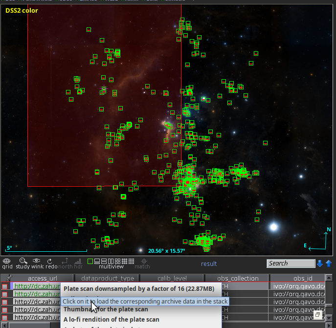
Investigating the spectra
The September post already discussed a few aspects of array plotting.
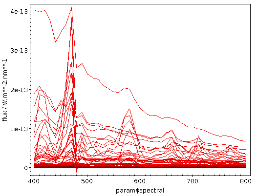
In short: try the plane plot and an XYArray control. Modern TOPCATs
(and for what I'm doing here it's wise to use something newer than
4.8-7) will automatically figure out suitable columns for the x and y
axes (except it forgets to label the spectral coordinate with its unit,
nm):
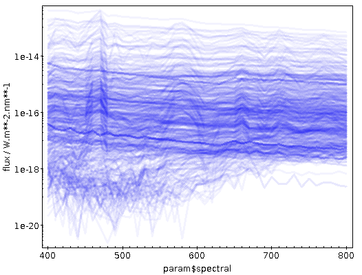
There's a quite a bit of crowding here; finding global characteristics
perhaps works better when you switch the ordinate to logarithmic, use
transparent shading (in the Form tab) and raise the opaque limit a
bit. This could give you something like:
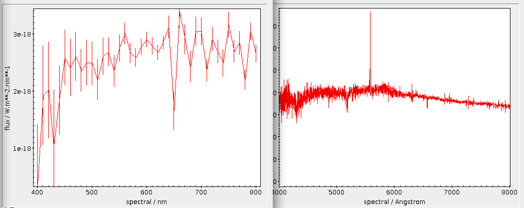
You can see that at least quite a few objects have nice and strong
emission lines, as I had hoped for when choosing WC stars for this
example. What if we could pick them out to build a template spectrum?
Well, let's try. With the new vector math in ADQL, the database can
normalise the spectra and compute a few statistics on them.
But first: In order to get rid of the source_id-computing CTE above, let
me obtain the source_ids I want to work with once and for all, as in:
SELECT source_id, main_id
FROM gaia.edr3lite AS l
  JOIN tap_upload.t1 AS u
        ON (DISTANCE(l.ra, l.dec, u.ra, u.dec)<0.001)
Memorise the Table List index of the result. With that, you can
directly work with the gdr3spec.spectra table and experiment a bit;
for me, the index was 10, and hence I use tap_uploads.t10 below.
Computing some statistics
The Gaia XP spectra are flux calibrated, and hence I will have to
normalise them if I want to compare them. Ignoring all errors and thus
in particular the fact that some (few) components are negative, this
normalisation is harmless: We just divide by the sum of all vector
components. The net result is that, were our spectra continuous, the
integral over them would be one. And let's then use the standard
deviation and the value of the 19th array element as metrics:
WITH normalised AS (
SELECT source_id, main_id,
        flux/arr_sum(flux) as nflux, flux
FROM gdr3spec.spectra
JOIN tap_upload.t10
USING (source_id))
SELECT
  source_id, main_id,
  flux, nflux,
  arr_avg(nflux*nflux)-POWER(arr_avg(nflux),2) AS sd,
  nflux[19] as em
FROM normalised
You can see quite a bit of the vector extension here:
- arr_sum and arr_avg: These work as the aggregate functions in
SQL do, just not on tuples but on the components of the vectors.
- Multiplication of vectors is element-wise, so nflux*nflux
computes a vector of the squares of the components of nflux.
That's also true for all other basic arithmetic operators. If you
know numpy: same thing.
- You fetch individual elements in the [] notation you probably know
from Python or C. Contrary to Python and C, common SQL
implementations count indexes from 1 by default, and we are keeping
that here (for now). Fortran lovers rejoice!
Why did I use nflux[19]? Well, there is a reasonably strong emission
feature in many spectra at about 580 nm (it's three-time ionised
carbon, or C IV in the rotten notation I usually apologise for when
talking to non-astronomers), which is, as experts tell me (thanks,
Andreas!), rather characteristic for the WC stars that I'm after
(whereas the even stronger feature on the left, around 470 nm, can also
be Helium).
If you inspect the spectral coordinate
that TOPCAT has on the abscissa (it's a param, so you'll have to go to
Views → Table Parameters to see it), you will see that each
spectral bin is 10 nm wide. So, I will hopefully hit the 580 nm feature
when fetching the 19th element of the spectral vector.
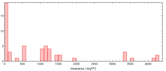
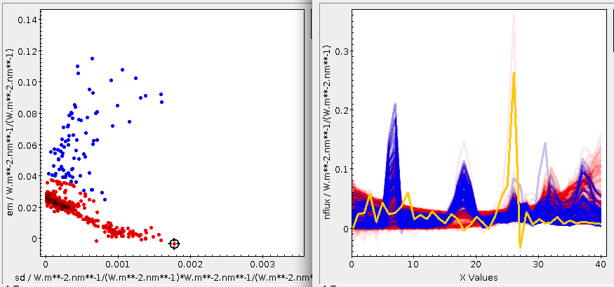
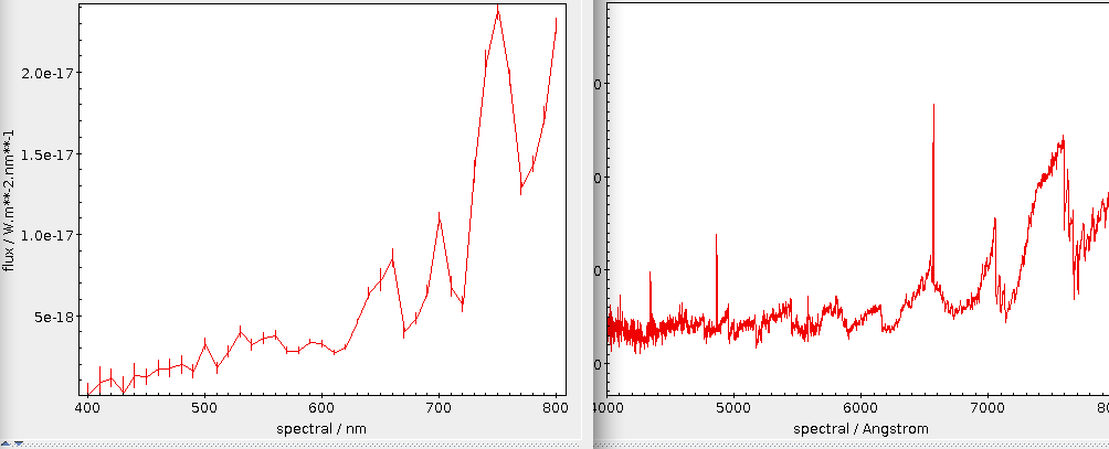
If you plot em versus the sd obtained like that, you will see
two reasonably distinct groups, where the ascending arm has relatively strong
emission around 580 nm and the descending arm does not. I have used the Blob
subset feature to select the upper arm into a subset ”upper” that is
blue in the following plot. If you click around in the em-sd plot and
show the Activated subset in an array plot, you can see things like:
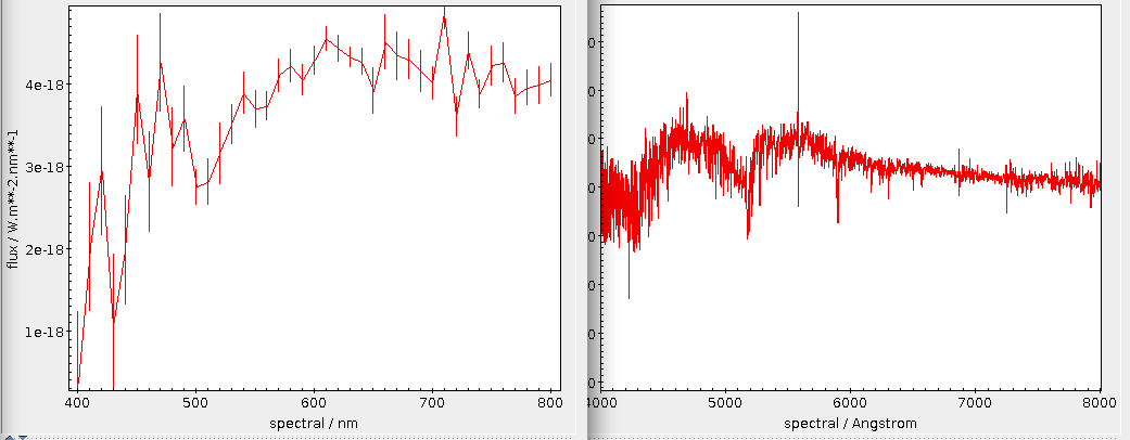
The activated spectrum (shown here in yellow) has a strong Hα but
basically no C IV – and it's safely outside of our carbon subset. Click
around a bit on the ascending arm, and you will see that all these
spectra have a bump around array element 18 (in TOPCAT's count, which
starts at 0).
Computing a Template on the Server Side
Whatever the subset of stars that we would like to use to define our
group of interest, we would now like to create a template spectrum from
them. A plausible way to do that is to sum them all up – that has the
nice side effect that stronger sources (which hopefully are less noisy)
have a larger weight.
To compute the template, in the Views → Column Info for the sd/em table,
unselect all columns but source_id (that way, you only upload what you
absolutely must), and in the main window, select the upper subset in
the Row Subset combo box. That way, only the rows in that subset will
get uploaded in the following query:
SELECT summed/arr_sum(summed) AS tpl
FROM (
  SELECT SUM(flux) AS summed
  FROM gdr3spec.spectra
  JOIN tap_upload.t19
  USING (source_id)) AS q
Again, you will have to adapt the t19 to where your manipulated
sd/em table is. If you get an “ambiguous column flux” error (or so)
here, you forgot to unselect all columns but source_id in the columns
window.
It pays to briefly appreciate what happens here: The SELECT
SUM(flux) is an aggregate function over arrays, meaning that all the
arrays are being summed over component-wise. Against that, the sum in
summed/arr_sum(summed) is summing within the array. If it helps
you, you could imagine having all the arrays in the table stacked.
Then, SUM(arr) produces the vertical margin sum, and
array_sum(arr) procudes the horizontal margin sum.
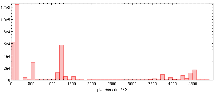
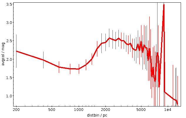
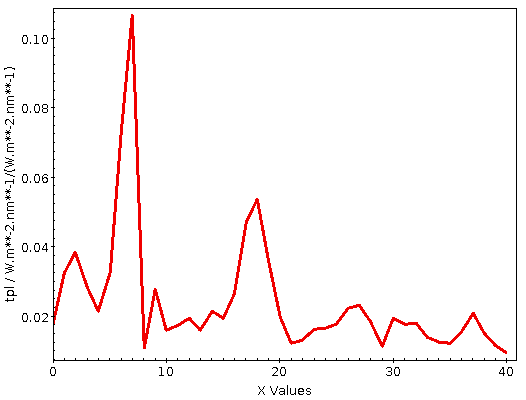
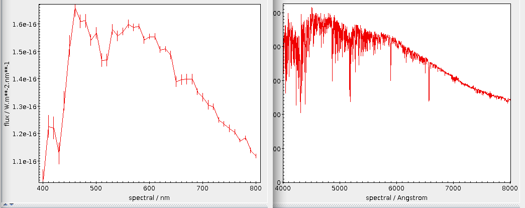
Well, here's the template I got in this way:
I give you that in this particular case, you could easily have done the
computation on the client side, because you already had the spectra in
your table. But the technique also works when you don't, and it will
scale to millions of arrays (although you will have to carefully think
about numerics when doing such enormous sums).
Also – I cannot lie – I simply had to have a pretext for showing you
aggregate functions over arrays.
Finding Similar Objects
Now that we have the template, can we find objects that have similar
properties? Sure: We upload the array and compute some metric, perhaps
the (squared) euclidian distances to normalised spectra. If the
template is in TOPCAT's table 25, you can write:
SELECT TOP 200000
  source_id,
  arr_sum(
    arr_map(
      power(x,2),tpl-flux/arr_sum(flux))) AS dist2,
  arr_sum(flux_error/flux) AS errs
FROM gdr3spec.spectra, tap_upload.t25
This will compute the distances between (conceptually randomly drawn)
200000 spectra and your template. I am also requesting the sum of the
(relative) flux errors
as a measure of how likely it is that wild wiggles actually are just
artefacts.
There is one array-related feature in that query I have not yet
mentioned: arr_map. This applies an expression to all components to
a vector, pretty much like python's map function, and my attempt to have
some (perhaps somewhat lame) substitute for numpy's ufunctions.
I am rather sure we really need something like this. SQL has no notion
of defining functions in queries. That is usually welcome, as otherwise
it would quicky become Turing-complete, which would be bad for what it
is designed to do. Here, however, that is a problem, because we do not
have a clean way to write the expression be be computed for each
component. For now, I have decreed that the first argument of map is an
expression over a formal x. This is ugly not only because it will be
confusing when there's an actual x in a table or query. I suspect with
a bit more thought and creativity, one can find a better solution that
still does not require a re-write of half the SQL grammar. But then
let's see – perhaps this makeshift hack proves to be less troublesome
than I expect.
Note that on my server, you will only get back 20000 matches by default;
you would have to adapt Max Rows to actually retrieve 200'000, and
then you also must switch to Asynchronous mode. This will then actually
take a non-trivial amount of CPU and disk I/O; going through the entire
set of 2e8 rows will be a matter of hours or so. Hence, I'm grateful if
you do all-sky scans only after having tested your queries on much
smaller subsets.
I've done this for 500'000 rows (which took a few minutes),
which might bring up a few C
IV-strong WR stars (these beasts are rare, you know).
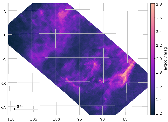
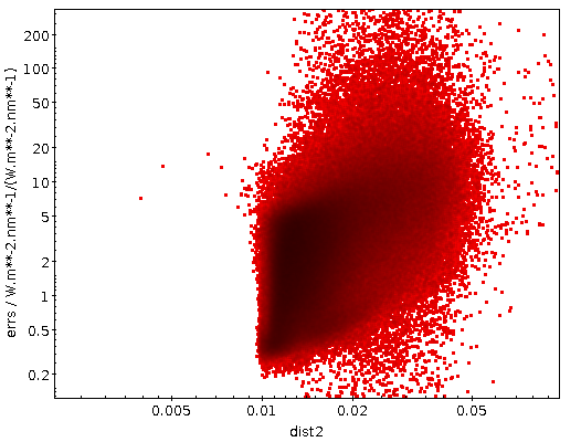
The result in the dist2/errs plane is (logplot
zoomed a bit):
Well: at least there are a few promising cases. Which would conclude
this little demo for the ADQL vector proposal. Looking at what we have
found here is another story.
Still, I could not resist having another look at what my box has found
there. There is a rather clear cut in the plot at perhaps 0.009,
and thus I created a
subset interesting consisting of objects for which dist2<0.009
(which is 18
objects for me) and did the trick above, only uploading
this interesting subset with only the source_id column to resolve to
Gaia DR3 (lite) rows:
SELECT *
FROM gaia.dr3lite
JOIN tap_upload.t33
USING (source_id)
And then I wondered whether any of these were known to SIMBAD and
switched to their TAP service:
SELECT
  tc.*, otype
FROM basic AS db
 RIGHT OUTER JOIN TAP_UPLOAD.t34 AS tc
 ON 1=CONTAINS(POINT('ICRS', db.ra, db.dec),
               CIRCLE('ICRS', tc.ra, tc.dec, 1./3600.))
Note the use of RIGHT OUTER JOIN to ensure we won't lose any matches on
the way; if this weren't such a small table, you'd be better off just
uploading the positions and then doing a local match to recover the rest
of the table, by the way.
As to what's coming back: Well, a bunch of white dwarf candidates, a
“blue“ star, a few objects SIMBAD knows as quasars (that at least makes
sense, because it's rather likely that some of them have lines
redshifted into my C IV window), and a few unclassified
objects. Whether SIMBAD is wrong on at least some of them,
whether the positional crossmatch fetched unrelated objects, or whether
I got it all wrong I will not decide here. Let me give you my candidates
as a VOTable, though.
You now know what you have to do to add nice, if low-resolution, spectra
to them.
Slices?
A notable absence from the current vector extension is slicing. I think
we should have it – in this example, this would be really useful when
summing different spectral regions without having to write long sums
(“synthetic broadband photometry“).
I have not put it in yet mainly because I am not sure if Python-like
syntax (nflux[4:7]) is a good idea when we have 1-based arrays.
Also: Do we want to keep the upper index out? That's certainly the
right thing for Python (where you want a[:3]+a[3:] == a), but is it
here? Speaking of which: Should we require support of half-open slices?
Should we rather have a function arr_slice? With what arguments?
I'd be curious about other peoples' thoughts on slicing.

![[RSS]](../theme/image/rss.png)