Articles from Data

• Find Outliers using ADQL and TAP

  2018-10-10 Markus Demleitner

  

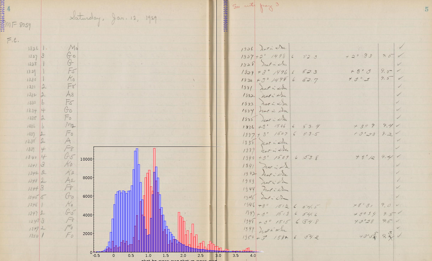
  Two pages from Annie Cannon's notebooks[1], and a histogram of the basic BP-RP color distribution in the HD catalogue (blue) and the distribution of the outliers (red). For more of Annie Cannon's notebooks, search on ADS.

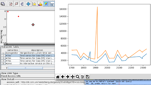
  The other day I gave one of my improvised live demos (“What, roughly, are you working on?”) and I ended up needing to translate identifiers from the Henry Draper Catalogue to modern positions. Quickly typing “Henry Draper” into TOPCAT's TAP search window didn't yield anything useful (some resources only using the HD, and a TAP service that didn't support uploads – hmpf).

  Now, had I tried the somewhat more thorough WIRR Registry interface, I'd have noted the HD catalogue at VizieR and in particular Fabricius' et al's HD-Tycho 2 match (explaining why they didn't show up in TOPCAT is a longer story; we're working on it). But alas, I didn't, and so I set out to produce a catalogue matching HD and Gaia DR2, easily findable from within TOPCAT's TAP client. Well, it's here in the form of the hdgaia.main table in our data center.

  Considering the nontrivial data discovery and some yak shaving I had to do to get from HD identifiers to Gaia DR2 ones, it was perhaps not as futile an exercise as I had thought now and then during the preparation of the thing. And it gives me the chance to show a nice ADQL technique to locate outliers.

  In this case, one might ask: Which objects might Annie Cannon and colleagues have misclassified? Or perhaps the objects have changed their spectrum between the time Cannon's photographic plates have been taken and Gaia observed them? Whatever it is: We'll have to figure out where there are unusual BP-RPs given the spectral type from HD.

  To figure this out, we'll first have to determine what's “usual”. If you've worked through our ADQL course, you know what to expect: grouping. So, to get a table of average colours by spectral type, you'd say (all queries executable on the TAP service at http://dc.g-vo.org/tap):

  select spectral,
    avg(phot_bp_mean_mag-phot_rp_mean_mag) as col,
    count(*) as ct
  from hdgaia.main
  join gaia.dr2light
  using (source_id)
  group by spectral
  

  – apart from the join that's needed here because we want to pull photometry from gaia, that's standard fare. And that join is the selling point of this catalog, so I won't apologise for using it already in the first query.

  The next question is how strict we want to be before we say something that doesn't have the expected colour is unusual. While these days you can rather easily use actual distributions, at least for an initial analysis just assuming a Gaussian and estimating its FWHM as the standard deviation works pretty well if your data isn't excessively nasty. Regrettably, there is no aggregate function STDDEV in ADQL (you could still ask for it: head over to the DAL mailing list before ADQL 2.1 is a done deal!). However, you may remember that Var(X)=E(X²)-E(X)², that the average is an estimator for the expectation, and that the standard deviation is actually an estimator for the square root of the variance. And that these estimators will work like a charm if you're actually dealing with Gaussian data.

  So, let's use that to compute our standard deviations. While we are at it, throw out everything that's not a star[2], and ensure that our groups have enough members to make our estimates non-ridiculous; that last bit is done through a HAVING clause that essentially works like a WHERE, just for entire GROUPs:

  select spectral,
    avg(phot_bp_mean_mag-phot_rp_mean_mag) as col,
    sqrt(avg(power(phot_bp_mean_mag-phot_rp_mean_mag, 2))-
      power(avg(phot_bp_mean_mag-phot_rp_mean_mag), 2)) as sig_col,
    count(*) as ct
  from hdgaia.main
  join gaia.dr2light
    using (source_id)
  where m_v<18
  group by spectral
  having count(*)>10
  

  This may look a bit scary, but if you read it line by line, I'd argue it's no worse than our harmless first GROUP BY query.

  From here, the step to determine the outliers isn't big any more. What the query I've just written produces is a mapping from spectral type to the means and scales (“µ,σ” in the rotten jargon of astronomy) of the Gaussians for the colors of the stars having that spectral type. So, all we need to do is join that information by spectral type to the original table and then see which actual colors are further off than, say, three sigma. This is a nice application of the common table expressions I've tried to sell you in the post on ADQL 2.1; our determine-what's-usual query from above stays nicely separated from the (largely trivial) rest:

  with standards as (select spectral,
    avg(phot_bp_mean_mag-phot_rp_mean_mag) as col,
    sqrt(avg(power(phot_bp_mean_mag-phot_rp_mean_mag, 2))-
      power(avg(phot_bp_mean_mag-phot_rp_mean_mag), 2)) as sig_col,
    count(*) as ct
    from hdgaia.main
    join gaia.dr2light
    using (source_id)
    where m_v<18
    group by spectral
    having count(*)>10)
  select *
  from hdgaia.main
  join standards
  using (spectral)
  join gaia.dr2light using (source_id)
  where
    abs(phot_bp_mean_mag-phot_rp_mean_mag-col)>3*sig_col
    and m_v<18
  

  – and that's a fairly general pattern for doing an initial outlier analysis on the the remote side. For HD, this takes a few seconds and yields 2722 rows (at least until we also push HDE into the table). That means you can keep 99% of the rows (the boring ones) on the server and can just pull the ones that could be interesting. These 99% savings aren't terribly much with a catalogue like the HD that's small by today's standards. For large catalogs, it's the difference between a download of a couple of minutes and pulling data for a day while frantically freeing disk space.

  By the way, that there's only 2.7e3 outliers among 2.25e5 objects, while Annie Cannon, Williamina Fleming, Antonia Maury, Edward Pickering, and the rest of the crew not only had to come up with the spectral classification while working on the catalogue but also had to classify all these objects manually. This is an amazing feat even if all of those rows actually were misclassifications (which they certainly aren't) – the machine classifiers of today would be proud to only get 1% wrong.

  The inset in the facsimile of Annie Cannons notebooks above shows how the outliers are distributed in color space relative to the full catalogue, where the basic catalogue is in blue and the outliers (scaled by 70) in red. Wouldn't it make a nice little side project to figure out the reason for the outlier clump on the red side of the histogram?

  [1]	The notebook pages are from a notebook Annie Cannon used in 1929. The material was kindly provided by Project PHAEDRA at the John G. Wolbach Library, Harvard College Observatory.

  [2]

  I'll not hide that I was severely tempted to undo the mapping of object classes to – for HD – unrealistic magnitudes (20 .. 50) but then left the HD as it came from ADC; I still doubt that decision was well taken, and sure enough, the example query above already has insane constraints on m_v reflecting that encoding. From today's position, of course there should have been an extra column or, better yet, a different catalogue for nonstellar objects. Ah well. It's always hard to break unhealty patterns.

• Deredden using TAP

  2018-08-17 Markus Demleitner

  

  Raw and dereddened CMD for a region in Cygnus.

  Today I published a nice new set of tables on our TAP service: The Bayestar17 3D dust map derived from Pan-STARRS 1 by Greg Green et al. I mention in passing that this was made particularly enjoyable because Greg and friends put an explicit license on their data (in this case, CC-BY-SA).

  This dust map is probably a fascinating resource by itself, but the really nifty thing is that you can use it to correct all kinds of photometric data for extinction – at least to some extent. On the Bayestar web page, the authors give some examples for usage – and with our new service, you can use TAP as well to correct photometry for extinction.

  To see how, first have a look at the table metadata for the prdust.map_union table; this is what casual users probably should look at. More specifically, at the coverage, best_fit, and grdiagnostic columns.

  coverage here is an interval of 10-healpixes. It has to be an interval because the orginal data comes on wildly different levels; depending on the density of stars, sometimes it takes the area of a 6-healpix (about a square degree) to get enough signal, whereas in the galactic plane a 10-healpix (a thousandth of a square degree) already has enough stars. To make the whole thing conveniently queriable without exploding a 6-healpix row into 1000 identical rows, larger healpixes translate into intervals of 10-helpixes. Don't panic, though, I'll show how to conveniently query this below.

  best_fit and grdiagnostic are arrays (remember the light cuves in Gaia DR2?). In bins of 0.5 in distance modulus (which is, in case you feel a bit uncertain as to the algebraic signs, 5 log10(dist)-5 for a distance in parsec), starting with a distance modulus of 4 and ending with 19. This means that for a distance modulus of 4.2 you should check the array index 0, whereas 4.3 already would be covered by array index 1. With this, best_fit[ind] gives E(B-V) = (B-V) - (B-V)₀ in the direction of coverage in a distance modulus bin of 2*ind+4. For each best_fit[ind], grdiagnostic[ind] contains a quality measure for that value. You probably shouldn't touch the E(B-V) if that measure is larger than 1.2.

  So, how does one use this?

  To try things, let's pull some Gaia data with distances; in order to have interesting extinctions, I'm using a patch in Cygnus (RA 288.5, Dec 2.3). If you live on the northern hemisphere and step out tonight, you could see dust clouds there with the naked eye (provided electricity fails all around, that is). Full disclosure: I tried the Coal Sack first but after checking the coverage of the dataset – which essentially is the sky north of -30 degrees – I noticed that wouldn't fly. But stories like these are one reason why I'm making such a fuss about having standard STC coverage representations.

  We want distances, and to dodge all the intricacies involved when naively turning parallaxes to distances discussed at length in a paper by Xavier Luri et al (and elsewhere), I'm using precomputed distances from Bailer-Jones et al. (2018AJ....156...58B); you'll find them on the "ARI Gaia" service; in TOPCAT's TAP dialog simply search for “Gaia” – that'll give you the GAVO DC TAP search, too, and that we'll need in a second.

  The pre-computed distances are in the gaiadr2_complements.geometric_distance table, which can be joined to the main Gaia object catalog using the source_id column. So, here's a query to produce a little photometric catalog around our spot in Cygnus (we're discarding objects with excessive parallax errors while we're at it):

  SELECT
  r_est, 5*log10(r_est)-5 as dist_mod,
  phot_g_mean_mag, phot_bp_mean_mag, phot_rp_mean_mag,
  ra, dec
  FROM
  gaiadr2.gaia_source
  JOIN gaiadr2_complements.geometric_distance
  USING (source_id)
  WHERE
  parallax_over_error>1
  AND 1=CONTAINS(POINT('ICRS', ra, dec), CIRCLE('ICRS', 288.5, 2.3, 0.5 ))
  

  The color-magnitude diagram resulting from this is the red point cloud in the animated GIF at the top. To reproduce it, just plot phot_bp_mean_mag-phot_rp_mean_mag against phot_g_mean_mag-dist_mod (and invert the y axis).

  De-reddening this needs a few minor technicalities. The most important one is how to match against the odd intervals of healpixes in the prdust.map_union table. A secondary one is that we have only pulled equatorial coordinates, and the healpixes in prdust are in galactic coordinates.

  Computing the healpix requires the ivo_healpix_index ADQL user defined function (UDF) that you may have met before, and since we have to go from ICRS to Galactic it requires a fairly new UDF I've recently defined to finally get the discussion on having a “standard library” of astrometric functions in ADQL going: gavo_transform. Here's how to get a 10-healpix as required for map_union from ra and dec:

  CAST(ivo_healpix_index(10,
    gavo_transform('ICRS', 'GALACTIC', POINT(ra, dec))) AS INTEGER)
  

  The CAST call is a pure technicality – ivo_healpix_index returns a 64-bit integer, which I can't use in my interval logic.

  The comparison against the intervals you could do yourself, but as argued in Registry-STC article this is one of the trivial things that are easy to get wrong. So, let's use the ivo_interval_overlaps UDF; it goes in the join condition to properly match prdust healpixes to catalog positions. Then our total query – that, I hope, should be reasonably easy to adapt to similar problems – is:

  WITH sources AS (
    SELECT phot_g_mean_mag,
      phot_bp_mean_mag,
      phot_rp_mean_mag,
      dist_mod,
      CAST(ivo_healpix_index(10,
        gavo_transform('ICRS', 'GALACTIC', POINT(ra, dec))) AS INTEGER) AS hpx,
      ROUND((dist_mod-4)*2)+1 AS dist_mod_bin
    FROM TAP_UPLOAD.T1)
  
  SELECT
    phot_bp_mean_mag-phot_rp_mean_mag-dust.best_fit[dist_mod_bin] AS color,
    phot_g_mean_mag-dist_mod+
      dust.best_fit[dist_mod_bin]*3.384 AS abs_mag,
    dust.grdiagnostic[dist_mod_bin] as qual
  FROM sources
  JOIN prdust.map_union AS dust
  ON (1=ivo_interval_has(hpx, coverage))
  

  (If you're following along: you have to switch to the GAVO DC TAP to run this, and you will probably have to change the index after TAP_UPLOAD).

  Ok, in the photometry department there's a bit of cheating going on here – I'm correcting Gaia B-R with B-V, and I'm using the factor for Johnson V to estimate the extinction in Gaia G (if you're curious where that comes from: See the footnote on best_fit and the MC extinction service docs should get you started), so this is far from physically correct. But, as you can see from the green cloud in the plot above, it already helps a bit. And if you find out better factors, by all means let me know so I can add an update... right here:

  Update (2018-09-11): The original data creator, Gregory Green points out that the thing with having a better factor for Gaia G isn't that simple, because, as he says “Gaia G is very broad, [and] the extinction coefficients are much more dependent on stellar type, and extinction is also more nonlinear with dust column (extinction is only linear with dust column and independent of stellar type for an infinitely narrow passband)”. So – when de-reddening, prefer narrow passbands. But whether narrow or wide: TAP helps you.

• Gaia DR2: A light version and light curves

  2018-05-07 Markus Demleitner

  

  Topcat is doing datalink, and our little python script has plotted a two-color time series of RMC 18 (or so I think).

  If anyone ever writes a history of the VO, the second data release of Gaia on April 25, 2018 will probably mark its coming-of-age – at least if you, like me, consider the Registry the central element of the VO. It was spectacular to view the spike of tens of Registry queries per second right around 12:00 CEST, the moment the various TAP services handing out the data made it public (with great aplomb, of course).

  In GAVO's Data Center we also carry Gaia DR2 data. Our host institute, the Zentrum für Astronomie in Heidelberg, also has a dedicated Gaia server. This gives relieves us from having to be a true mirror of the upstream data release. And since the source catalog has lots and lots of columns that most users will not be using most of the time, we figured a “light” version of the source catalog might fill an interesting ecological niche: Behold gaia.dr2light on the GAVO DC TAP service, containing essentially just the basic astrometric parameters and the diagonal of the covariance matrix.

  That has two advantages: Result sets with SELECT * are a lot less unwieldy (but: just don't do this with Gaia DR2), and, more importantly, a lighter table puts less load on the server. You see, conventional databases read entire rows when processing data, and having just 30% of the columns means we will be 3 times faster on I/O-bound tasks (assuming the same hardware, of course). Hence, and contrary to several other DR2-carrying sites, you can perform full sequential scans before timing out on our TAP service on gaia.dr2light. If, on the other hand, you need to do debugging or full-covariance-matrix error calculations: The full DR2 gaia_source table is available in many places in the VO. Just use the Registry.

  Photometry via TAP

  A piece of Gaia DR2 that's not available in this form anywhere else is the lightcurves; that's per-transit photometry in the G, BP, and RP band for about 0.5 million objects that the reduction system classified as variable. ESAC publishes these through datalink from within their gaia_source table, and what you get back is a VOTable that has the photometry in the three bands interleaved.

  I figured it might be useful if that data were available in a TAP-queriable table with lightcurves in the database. And that's how gaia.dr2epochflux came into being. In there, you have three triples of arrays: the epochs (g_transit_time, bp_obs_time, and rp_obs_time), the fluxes (g_transit_flux, bp_flux, and rp_flux), and their errors (you can probably guess their names). So, to retrieve G lightcurves where available together with a gaia_source query of your liking, you could write something like:

  SELECT g.*, g_transit_time, g_transit_flux
  FROM gaia.dr2light AS g
  LEFT OUTER JOIN gaia.dr2epochflux
  USING (source_id)
  WHERE ...whatever...
  

  – the LEFT OUTER JOIN arranges things such that the g_transit_time and g_transit_flux columns simply are NULL when there are no lightcurves; with a normal (“inner”) join, rows without lightcurves would not be returned in such a query.

  To give you an idea of what you can do with this, suppose you would like to discover new variable blue supergiants in the Gaia data (who knows – you might discover the precursor of the next nearby supernova!). You could start with establishing color cuts and train your favourite machine learning device on light curves of variable blue supergiants. Here's how to get (and, for simplicity, plot) time series of stars classified as blue supergiants by Simbad for which Gaia DR2 lightcurves are available, using pyvo and a little async trick:

  from matplotlib import pyplot as plt
  import pyvo
  
  def main():
    simbad = pyvo.dal.TAPService(
      "http://simbad.u-strasbg.fr:80/simbad/sim-tap")
    gavodc = pyvo.dal.TAPService("http://dc.g-vo.org/tap")
  
    # Get blue supergiants from Simbad
    simjob = simbad.submit_job("""
      select main_id, ra, dec
      from basic
      where otype='BlueSG*'""")
    simjob.run()
  
    # Get lightcurves from Gaia
    try:
      simjob.wait()
      time_series = gavodc.run_sync("""
        SELECT b.*, bp_obs_time, bp_flux, rp_obs_time, rp_flux
        FROM (SELECT
           main_id, source_id, g.ra, g.dec
           FROM
          gaia.dr2light as g
           JOIN TAP_UPLOAD.t1 AS tc
           ON (0.002>DISTANCE(tc.ra, tc.dec, g.ra, g.dec))
        OFFSET 0) AS b
        JOIN gaia.dr2epochflux
        USING (source_id)
        """,
        uploads={"t1": simjob.result_uri})
    finally:
      simjob.delete()
  
    # Now plot one after the other
    for row in time_series.table:
      plt.plot(row["bp_obs_time"], row["bp_flux"])
      plt.plot(row["rp_obs_time"], row["rp_flux"])
      plt.show(block=False)
      raw_input("{}; press return for next...".format(row["main_id"]))
      plt.cla()
  
  if __name__=="__main__":
    main()
  

  If you bother to read the code, you'll notice that we transfer the Simbad result directly to the GAVO data center without first downloading it. That's fairly boring in this case, where the table is small. But if you have a narrow pipe for one reason or another and some 10⁵ rows, passing around async result URLs is a useful trick.

  In this particular case the whole thing returns just four stars, so perhaps that's not a terribly useful target for your learning machine. But this piece of code should get you started to where there's more data.

  You should read the column descriptions and footnotes in the query results (or from the reference URL) – this tells you how to interpret the times and how to make magnitudes from the fluxes if you must. You probably can't hear it any more, but just in case: If you can, process fluxes rather than magnitudes from Gaia, because the errors are painful to interpret in magnitudes when the fluxes are small (try it!).

  Note how the photometry data is stored in arrays in the database, and that VOTables can just transport these. The bad news is that support for manipulating arrays in ADQL is pretty much zero at this point; this means that, when you have trained your ML device, you'll probably have to still download lots and lots of light curves rather than write some elegant ADQL to do the filtering server-side. However, I'd be highly interested to work out how some tastefully chosen user defined functions might enable offloading at least a good deal of that analysis to the database. So – if you know what you'd like to do, by all means let me know. Perhaps there's something I can do for you.

  Incidentally, I'll talk a bit more about ADQL arrays in a blog post coming up in a few weeks (I think). Don't miss it, subscribe to our feed).

  Datalink

  In the results from queries involving gaia.dr2epochflux, we also provide datalinks. These let you retrieve lightcurves that already have mags and that are more easily plotted. Perhaps more importantly, they link back to the full ESAC lightcurves that, in addition, give you a lot more debug information and are required if you want to reliably identify photometry points with the identifiers of the transits that generated them.

  Datalink support in clients still is not great, but it's growing nicely. Your ideas for workflows that should be supported are (again) most welcome – and have a good chance of being adopted. So, try things out, for instance by getting the most recent TOPCAT (as of this writing) and do the following:

  1. Open the VO/TAP dialog from the menu bar and double click the GAVO DC TAP service.

  2. Enter:

       SELECT source_id, ra, dec,
       phot_bp_mean_mag, phot_rp_mean_mag, phot_g_mean_mag,
       g_transit_time, g_transit_flux,
       rp_obs_time, rp_flux
       FROM gaia.dr2epochflux
       JOIN gaia.dr2light
       USING (source_id)
       WHERE parallax>50
     
     into “ADQL” text to retrieve lightcurves for the more nearby
     variables (in reality, you'd have to be a bit more careful with the
     distances, but you already knew that).
     

  3. plot something like phot_bp_mean_mag-phot_rp_mean_mag vs. phot_g_mean_mag (and adapt the plot to fit your viewing habits).

  4. Open the dialog for Views/Activation Actions (from the menu bar or the tool bar – same thing), check “Invoke Service”, choose “View Datalink Table”.

  5. Whenever you click on a a point in your CMD, a window will pop up in which you can choose between the time series in the various bands, and you can pull in the data from ESAC; to load a table, select “Load Table” from the actions near the foot of the datalink table and click “Invoke”.

  Yeah. It's clunky. Help us make it better with your fresh ideas for interfaces (and don't be cross with us if we have to marry them with what's technically feasible and readily generalised).

  SSAP and Obscore

  If you're fed up with bleeding-edge tech, the light curves are also available through good old SSAP and Obscore. To use that, just get Splat (or another SSA client, preferably with a bit of time series support). Look for a Gaia DR2 time series service (you may have to update the service list before you find it), enter (in keeping with our LBV theme) S Dor as position and hit “Lookup” followed by “Send Query”. Just click on any result to just view the time series – and then apply Splat's rich tool set to it.

  Update (8.5.2018): Clusters

  Here's another quick application – how about looking for variable stars in clusters? This piece of ADQL should get you started:

  SELECT TOP 100
    source_id, ra, dec, parallax, g.pmra, g.pmdec,
    m.name, m.pmra AS c_pmra, m.pmde AS c_pmde,
    m.e_pm AS c_e_pm,
    1/dist AS cluster_parallax
  FROM
    gaia.dr2epochflux
    JOIN gaia.dr2light AS g USING (source_id)
    JOIN mwsc.main AS m
    ON (1=CONTAINS(
      POINT(g.ra, g.dec),
      CIRCLE(m.raj2000, m.dej2000, rcluster)))
  WHERE IN_UNIT(pmdec, 'deg/yr') BETWEEN m.pmde-m.e_pm*3 AND m.pmde+m.e_pm*3
  

  – yes, you'll want to constrain pmra, too, and the distance, and properly deal with error and all. But you get simple lightcurves for free. Just add them in the SELECT clause!

• The Earth is Our Telescope

  2017-07-31 Markus Demleitner

  

  The coverage of the 2007-2012 Antares neutrinos, with positional uncertainties scaled by three.

  At our Heidelberg data center, we have have already published some neutrino data, for instance the Amanda-II neutrino candiates, the IceCube-40 neutrino candidates, and the 2007-2010 Antares results.

  That latter project has now given us updated data, for the first time including timestamps, available as the Antares service.

  Now, if you look at the coverage (above), you'll notice at least two things: For one, there's no data around the north pole. That's because the instrument sits beyond the waters of the Mediterranean sea, not far from where some of you may now enjoy your vacation. And it is using the Earth as its filter – it's measuring particles as they come ”up” and discards anything that goes “down”. Yes, neutrinos are strange beasts.

  The second somewhat unusual thing is that the positional uncertainties are huge compared to what we're used to from optical catalogs: a degree is not uncommon (we've scaled the error circles by a factor of 3 in the image above, though). And that requires some extra care when working with the data.

  In our table, we have a column origin_est that actually contains circles. Hence, to find images of the “strongest” neutrinos in our obscore table, you could write:

  SELECT * FROM
  ivoa.obscore AS o
  JOIN (
    SELECT top 10 * FROM antares.data
    ORDER BY n_hits desc
  ) AS n
  ON 1=INTERSECTS(
    s_region,
    origin_est)
  

  in a query to our TAP service.

  But of course, this only gets really exciting when you can hope that perhaps that neutrino was emitted by some violent event that may have been observed serendipitously by someone else. That query then is (and we're using all the neutrinos now):

  SELECT * FROM
  ivoa.obscore AS o
  JOIN antares.data as n
  ON
     epoch_mjd between t_min-0.01 and t_max+0.01
    AND
      dataproduct_type='image'
    AND
      1=INTERSECTS(origin_est, s_region)
  

  On our data center, this doesn't yield anything at the moment (it does, though, if you do away with the spatial constraint, which frankly suprised me a bit). But then if you went and ran this query against obscore services of active observatories? And perhaps had your computer try and figure out whether anything unusual is seen on whatever you find?

  We think that would be really nifty, and right after we've published a first version of our little pyVO course (which is a bit on the back burner, but watch this space), we'll probably work that out as a proper pyVO use case.

  And meanwhile: In case you'll be standing on the shores of the Mediterranean this summer, enjoy the view and think of the monster deep down in there waiting for neutrinos to detect – and eventually drop into our data center.

• See Who's Kinking the Sky

  2017-03-14 Markus Demleitner

  A new arrival in the GAVO Data Center is UCAC5, another example of a slew of new catalogs combining pre-existing astrometry with Gaia DR1, just like the HSOY catalog we've featured here a couple of weeks back.

  That's a nice opportunity to show how to use ADQL's JOIN operator for something else than the well-known CONTAINS-type crossmatch. Since both UCAC5 and HSOY reference Gaia DR1, both have, for each object, a notion which element of the Gaia source catalog they correspond to. For HSOY, that's the gaia_id column, in UCAC5, it's just source_id. Hence, to compare results from both efforts, all you have to do is to join on source_id=gaia_id (you can save yourself the explicit table references here because the column names are unique to each table.

  So, if you want to compare proper motions, all you need to do is to point your favourite TAP client's interface to http://dc.g-vo.org/tap and run:

  SELECT
      in_unit(avg(uc.pmra-hsoy.pmra), 'mas/yr') AS pmradiff,
      in_unit(avg(uc.pmde-hsoy.pmde), 'mas/yr') AS pmdediff,
      count(*) as n,
      ivo_healpix_index (6, raj2000, dej2000) AS hpx
      FROM hsoy.main AS hsoy
      JOIN ucac5.main as uc
      ON (uc.source_id=hsoy.gaia_id)
      WHERE comp IS NULL    -- hsoy junk filter
      AND clone IS NULL     -- again, hsoy junk filter
      GROUP BY hpx
  

  (see Taylor et al's All of the Sky if you're unsure what do make of the healpix/GROUP BY magic).

  Of course, the fact that both tables are in the same service helps, but with a bit of upload magic you could do about the same analysis across TAP services.

  Just so there's a colourful image in this post, too, here's what this query shows for the differences in proper motion in RA:

  (equatorial coordinates, and the aux axis is a bit cropped here; try for yourself to see how things look for PM in declination or when plotted in galactic coordinates).

  What does this image mean? Well, it means that probably both UCAC5 and HSOY would still putt kinks into the sky if you wait long enough.

  In the brightest and darkest points, if you waited 250 years, the coordinate system induced by each catalog on the sky would be off by 1 arcsec with respect to the other (on a sphere, that means there's kinks somewhere). It may seem amazing that there's agreement to at least this level between the two catalogs – mind you, 1 arcsec is still more than 100 times smaller than you could see by eye; you'd have to go back to the Mesolithic age to have the slightest chance of spotting the disagreement without serious optical aids. But when Gaia DR2 will come around (hopefully around April 2018), our sky will be more stable even than that.

  Of course, both UCAC5 and HSOY are, indirectly, standing on the shoulders of the same giant, namely Hipparcos and Tycho, so the agreement may be less surprising, and we strongly suspect that a similar image will look a whole lot less pleasant when Gaia has straightened out the sky, in particular towards weaker stars.

  But still: do you want to bet if UCAC5 or HSOY will turn out to be closer to a non-kinking sky? Let us know. Qualifications („For bright stars...”) are allowed.

« Page 3 / 4 »