![[RSS]](../theme/image/rss.png)
DASCH is now in the VO
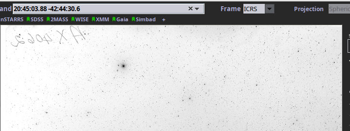
This frame would show comet 2P/Encke during its proximity to Earth in 1941 – if it went deep enough. But never mind practicalities: If you want to learn about matching ephemeris against the DASCH plate collection (or, really, any sort of obscore-like table), read on.
For about a century – that is, into the 1980s –, being an observational astronomer meant taking photographic plates and doing tricks with them (unless you were a radio astronomer or one of the very few astronomers peeking beyond radio and optical in those days, of course). This actually is somewhat fortunate for archivists, because unlike many of the early CCD observations that by now are lost with our ability to read the tapes they were stored on, the plates are still there.
Why Bother?
However, to make them usable, the plates need to be digitised. In the GAVO data centre, we keep the results of several scan campaigns large and small, such as HDAP, the various data collections joined in the historical photographic plate image archive HPPA, or the delightfully quirky Münster Flare Plates.
I personally care a lot about these data collections. This is partly because they are indispensible for understanding the history of astronomy. But more importantly, they are the next best thing we have to a time machine; if we have a way of knowing how the sky looked like seventy years ago, it is these plate collections. Having such a time machine is important for all kinds of scientific efforts, including figuring out whether there are aliens (i.e., 2016ApJ...822L..34S) on Tabby's Star.
Somewhat to my chagrin, the cited paper 2016ApJ...822L..34S did not use the VO to obtain the plate images but went straight to DASCH's web interface. DASCH, in case you have not heard of it before, is probably the most ambitious project concerned with plate digitisation at the moment – or perhaps: “was”, because they just finished scanning the core part of Harvard's plate collections, which was their primary goal.
I can understand why Bradley Schaefer, the paper's author, did not bother with a VO search In 2016. For starters, working with halfway homogeneous data from instruments you are somewhat familiar saves a substantial amount of work and thought, in particular if you are, in addition, up against the usual lack of machine-readable metadata. Also, at that time DASCH probably had about as many digitised plates as all the VO's contemporary plate collections taken together.
DASCH: The Harvard Plates
Given such stats, I have always wanted to have at least the metadata from DASCH's plates in the VO. Thanks to a recent update to DASCH's publication system, this is now a reality. Since 2024-04-29, I am publishing the metadata of the DASCH plates via Obscore and and SIAP2.
Followup (2024-05-03)
This is now DASCH news, and one of my two main contacts on the DASCH side, Peter Williams, has written an insightful post on this, too. Let me use this opportunity to thank him for the delightful cooperation, and extend these thanks to Ben Sabath, who is primarily responsible for the update to the DASCH publication system I mentioned above.
Matching plates are returned as datalink documents, pointing to a preview, photos of the plate and its jacket, and links to the science data, once downsampled by a factor of 16, once in the original size (example). For now, #this points to the downsampled version, as Amazon charges DASCH about three cents per full-scale plate at the moment, and that can quickly add up by accident (there's nothing wrong with consciously downloading full-scale FITS-es if you need them, of course).
This is a bit fishy in that the size of the image in the obscore/SIAP2 fields s_xel1 and s_xel2 refers to the unscaled image, and thus I should be returning the full-scale image as datalink #this. I hope I will not cause much confusion with this design.
In case you look at the links in the datalink documents, let me include a disclaimer: Although they point into the GAVO data centre, the data is served courtesy of the DASCH project. The links only go to us because we need to sign links for you. I mention this because you can save the datalink documents and the links within them; the URLs you are redirected to from there, however, will expire fast. Just do not look at them.
Followup (2025-02-05)
As of today, we support cutouts of DASCH plates, too. This is a fairly basic service at this point, returning fixed-size cutouts only. However, for many use cases, these cutouts may be good enough.
For instance, here is how to retrieve cutouts for the vicinity of M51:
import pyvo

pos = (202.46, 47.19)

svc = pyvo.dal.TAPService("http://dc.g-vo.org/tap")
res = svc.run_sync(f"""
    SELECT *
    FROM
        dasch.narrow_plates
    WHERE
        distance(s_ra, s_dec, {pos[0]}, {pos[1]})<0.5""")
for rec in res:
    prod = rec.processed(circle=pos+(0.1,))
    dest_name = rec["dasch_id"]+".cutout.fits"
    print(dest_name)
    with open(dest_name, "wb") as f:
        f.write(prod.data)
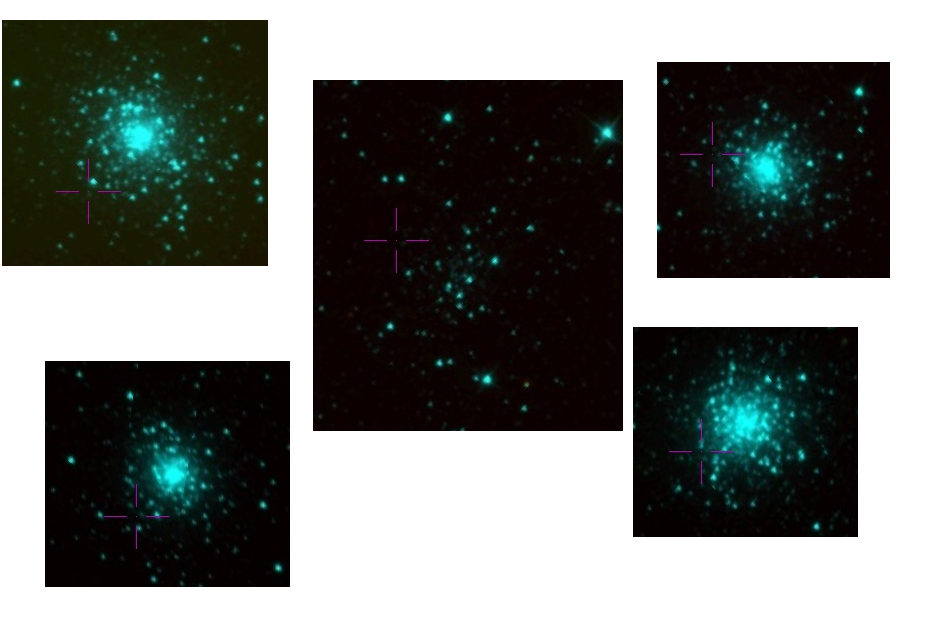
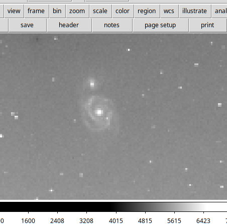
And this is what M51 looked like in 1968 through the 12-inch Metcalf Doublet (DASCH id ma11561), displayed in ds9:
Plates in Global Discovery
So – what can you do with DASCH in the VO that you could not do before?
Most importantly, you will discover DASCH in registry interfaces and its datasets in global queries (in particular the global dataset queries I have discussed a few weeks ago). For instance, DASCH is now in Aladin's discovery tree:
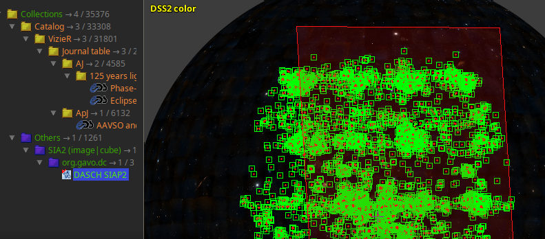
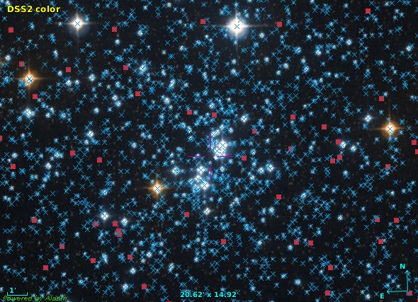
You can now find DASCH in Aladin and do the usual “in view“ searches. However, currently this yields many matches that are, in practical terms, spurious, as they come from extremely wide-angle instruments. The red rectangle is the footprint of one of these images; note that the view here is a full two pi sky. We will probably do something about this “noise“.
The addition of DASCH to the VO has a strong effect in some use cases. For instance, at the end of the GAVO plates tutorial, we do an all-VO obscore query that, at the time of the last update of the tutorial in 2019, yielded 4067 datasets (of course, including modern and/or non-optical observations) potentially showing some strongly lensed quasar. With DASCH – and, admittedly, a few more collections that came into the VO since 2019 –, that number is now 10'489; the range of observation dates grew from MJD 12550…52000 to MJD 9800…58600, with the mean decreasing from 51'909 to 30'603. That the mean observation date moves that much back in time is a certain sign that a major part of the expansion is due to DASCH (well, and certainly to APPLAUSE, too).
Followup (2024-05-03)
As discussed in my DASCH update, I have taken out the large-coverage plates from my obscore table, which changes the stats (but not the conclusions) quite a bit. They is now 10'098 plates and mean observation date 36'396
TAP, Uploads, and pyVO on DASCH
But this is not just about bringing astronomical heritage to the VO. It is also about exposing DASCH through the powerful ADQL/TAP interface. As an example of how this may be useful, consider the comet P2/Encke, which, according to JPL's Small-Body Database was relatively close to Earth (about half an AU) in May 1941. It would have had about 14.5 mag at that point and hence was safely within reach of several of the instruments archived in DASCH. Perhaps we can find serendipitous or even targeted observations of the comet in the collection?
The plan to find that out is: compute an ephemeris (we are lazy and use an external service, Miriade ephemcc) and then for each day see whether there are DASCH observations in the vicinity of the sky location obtained in this way.
As usual, it's never that easy because the call to the ephemeris webservice (paste the link into TOPCAT to have a look) returns cursed sexagesimal coordinates. We need to fix them before doing anything serious with the table, and while we are at it, we also repair the date, which is simpler to consume if it is MJD to begin with. Getting the ephemeris thus takes quite a few lines:
from astropy import table
from astropy import units as u
from astropy.coordinates import SkyCoord
from astropy.time import Time

ephem = table.Table.read(
  "https://vo.imcce.fr/webservices/miriade/ephemcc.php?-from=vespa"
  "&-name=c:p/encke&-ep=1941-04-01&-nbd=90&-step=1d&-observer=500"
  &-mime=votable")

parsed = SkyCoord(ephem["ra"], ephem["dec"], unit=(u.hourangle, u.deg))
ephem["ra"] = parsed.ra.degree
ephem["dec"] = parsed.dec.degree

parsed = Time(ephem["epoch"])
ephem["epoch"] = parsed.mjd
Compared to that, the actual matching against DASCH is almost trivial if you are somewhat familiar with crossmatching in ADQL and the Obscore schema:
svc = pyvo.dal.TAPService("http://dc.g-vo.org/tap")
res = svc.run_sync("""
    SELECT *
    FROM
        dasch.plates
        JOIN tap_upload.orbit
        ON (1=CONTAINS(POINT(ra, dec), s_region))
    WHERE
        t_min<epoch
        AND t_max>epoch""",
    uploads={"orbit": ephem})
Followup (2024-05-03)
You would probably query the dasch.narrow_plates table in actual operations; querying dasch.plates is probably more for people interested in the history of astronomy or DASCH itself.
Inspect the query for a moment: This is a normal upload join, except we are constructing an ADQL POINT on the fly to be able to see whether we are in the spatial region covered by a DASCH dataset (given in obscore's s_region column). We could have put the temporal condition into the join's ON; but I think the intention is somewhat clearer with the WHERE constraint, and the database engine will probably go through identical motions for both queries – the beauty of having a query planner in the loop is that you do not need to think about such details most of the time.
Actually, in this case there is one last complication: As said above, we have put a datalink service between you and the downloads to discourage accidental large downloads. We hence use pyVO's (suboptimally documented) datalink interface (iter_datalinks):
with pyvo.samp.connection() as conn:
    for dl in res.iter_datalinks():
        link = next(dl.bysemantics("#preview-image"))
        pyvo.samp.send_image_to(
            conn,
            link.access_url,
            client_name="Aladin")
Among the artefacts available we pick the scaled jpegs in this fragment (#preview-image), since these are almost free even on the Amazon cloud. Change that #preview-image to #this in the to get scaled calibrated FITS-es, which are still fairly small. This would, for instance, let you overplot the ephemeris in Aladin, which you cannot do with the jpegs as they lack astrometric calibration (for now). But even with #preview-image, we can use Aladin as a glorified image viewer by SAMP-sending the images there, which is why we do the minor magic with functions from pyvo.samp.
If you want to try this yourself or mangle the program to do something else that requires querying against a reasonable number positions in time and space, just get encke.py and hack away. Make sure to start Aladin before running the program so it has something to send the images to.
Disclaimers
This is a contrived example, and it is likely that this particular use case is astronomically wrong in several ways. Let me enumerate a few things that would need looking into before this approaches proper science:
- We compute the ephemeris for the center of the Earth. At half an AU distance, the resulting parallax will not shift the position enough to hide a plate we should know about, but at least for anything closer, you should try to do a bit better; admittedly, for a resource like DASCH – that contains plates from observatories all over the place – you will have to compromise.
- The ephemeris is probably wrong; comet's orbits change over time, and I have no idea if the ephemeris service actually uses 2P/Encke's 1941 orbit to compute the positions.
- The coordinate metadata may be wrong. Ephemcc's documentation says something that sounds a lot as if they were sometimes returning RA and Dec for the equator of the time rather than for J2000 (i.e., ICRS for all intents and purposes), but of course our obscore coverages are for the ICRS. Regrettably, the VOTable returned by the service does not contain a COOSYS element yet, and so there is no easy way to tell.
- If you look at the table with DASCH matches, you will see they all were observed with an extremely wide-angle instrument sporting an aperture of a mere three inches. Even at the whopping exposure times (two hours), there is probably no way you would see a diffuse object of 14th mag on a plate with a 1940s-era photographic emulsion with that kind of optics (well: feel free to prove me wrong).
- It would of course be a huge waste of bandwidth to pull the entire plates if we already had a good idea of where we would expect the comet (i.e., had a reliable ephemeris). Hence, a cutout service that would let you retrieve more or less exactly the pixels you would like to use for your research and not the cruft around it would be a nifty supplement. It's in the works, and I'd say you can almost hold your breath. The cutout will simply appear as a SODA service in the datalink documents. See 2020ASPC..522..295D for how you would operate such a service.