![[RSS]](./theme/image/rss.png)
Sofa instead of Granada
Gesticulating wildly to a computer is what happens in an online conference. To me, at least. Let's hope nobody watched me through the window.
It was already in the wee hours of Friday last week (CET) when the second "virtual Interop" had its rather unceremonious closing ceremony. Its predecessor in May had about it an air of a state of emergency. For instance, all sessions were monothematic. That was nice on the one hand, because a relatively large part of the time was available for discussion – which, really, is what the Interops are about. But then Interops are also about noticing what everyone else in the Virtual Observatory is cooking up, for which the short-ish talks we usually have at Interops work really well.
In contrast to that first Corona Interop, this second one, replacing what would have taken place in Granada, Spain, had a much more conventional format, which again accomodated many talks. But of course, this made one feel the lack of possibilities to quickly hash out a problem during a coffee break or in a spontaneous splinter quite a bit more.
Be that as it may, I would like to give you some insights on what I'm currently up to at the IVOA level; I am grateful for any feedback you can give on any of these topics.
Given that I currently chair the Semantics Working group, there was a natural focus on topics around vocabularies, and I gave two talks in that department. The one in DAL (DAL is the working group that builds the actual access protocols such as TAP or SIAP) was mainly on Datalink-related aspects of my Vocabularies in the VO 2 draft (VocInVO2), which in particular was an opportunity to thank everyone involved in the Vocabulary Enhancement Proposals we have been running this last year (all of which were about Datalink and hence closely tied to DAL). One thing I was asking for was reviews on a github pull request that would make the bysemantics method of Datalink accesses semantics-aware; basically, as intended by the original Datalink authors, when asking for #calibration links, this will also return, say, #bias links. If you can spare a moment for this: Please do!
Another thing I tried to raise some interest for is the proposed vocabulary of product types; this, I think, should eventually define what people may put into the dataproduct_type column of Obscore results, and there are related uses in Datalink and, believe it or not, the registration of SSAP (spectral) services. A question Alberto raised while I was discussing that made me realise I forgot to mention another vocabularies-related development relevant for DAL: I've put the gavo_vocmatch ADQL user-defined function into DaCHS. It lets you match something against a term or its narrower terms, referencing an IVOA vocabulary. For instance, if we had different sorts of time series (which, of course, would be odd for obscore that has the o_ucd column for this kind of thing), you could, using ADQL, still get all time series by querying:
SELECT TOP 5 *
FROM ivoa.obscore
WHERE
  1=gavo_vocmatch(
    ’product-type’,
    ’timeseries’,
    dataproduct_type)
Here, the first argument is the vocabulary name (whatever is after the http://www.ivoa.net/rdf in the vocabulary URL), the second the “root” term, and the third the column to match against. Since postgres, for now, isn't aware of IVOA vocabularies, the second argument must be a literal string rather than, say, an expression involving columns.
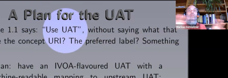
I gave a second semantics-related talk in the Registry session. That had its focus on the Unified Astronomy Thesaurus (UAT), from which people should pick the subject keywords in the VO Registry (actually, they should pick from its representation at http://www.ivoa.net/rdf/uat). I'll probably blog about that a little more some other time. For now, let me recommend a little UAT-based game on my Semantics Based Registry Browser sembarebro: Choose two terms that are pretty far apart (like, perhaps, ionized-coma-gases and cosmic-background-radiation) and then try to join the two sub-graphs. Warning: This may waste your time. But it will acquaint you with the UAT, which may be a good thing.
In that second talk, I also mentioned a second draft vocabulary I've put up in the past six months, http://www.ivoa.net/rdf/messenger. This builds upon the terms for VODataService's waveband element, which enumerated certain flavours of photons (like Radio, Optical, or X-ray). Now that we explore other messengers as well and have more and more solar system resources in the Registry, I'm arguing we ought to open up things by making “Photon” explicit in there and then adding Neutrinos and, later, other messengers. I've received a certain amount of pushback there on mixing the electromagnetic spectrum with particle types; on the other hand, the hierarchical nature of our vocabularies would, I think, let us smartly get away with that.
Speaking about solar system resources, I'm also listed as an author on Stéphane Erard's talk on EPN-TAP and EPNCore v2.0, probably due to my involvement in finally bringing EPN-TAP into the IVOA document repository. I've already talked about that in a 2017 post on this blog – and again, if you're interested in solar system data, this would be a good time to review the EPN-TAP working draft.
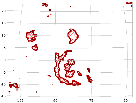
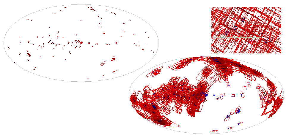
Talking about things regluar readers of this blog will have heard of: September's Crazy Shapes post I've referenced in a talk on MOCs in pgsphere, together with a fervent appeal to data centers to become involved in pgsphere maintenance.
And then there was my colleague Margarida's talk on LineTAP, a proposal to obsolete the little-used SLA protocol (which lets people search for spectral lines) with something combining the much more successful VAMDC with our beloved TAP. Me, I'm in this because I'd like to bring TOSS data closer to VAMDC – but also because having competing infrastructures for the same thing sucks.
And finally, I gave a talk I've called Data Model Posture Review in a session of the Data Models working group; I was somewhat worried that given its rather skeptical outlook it wouldn't be really well-received. But in fact quite a few people shared my main conclusions – and perhaps it was another step towards resolving my decade-old spot of pain: that the VO still doesn't offer tech to reliably bring two catalogues to the same epoch without human intervention.
With this number of talks I've been involved in, I'm essentially back to the level of a normal Interop. Which means I've been fairly knocked-out on Friday. And I can't lie: I still regret I didn't get to spend a few more warm days in Granada. Corona begone!